Population genomics statistics • ggPopi

ggpop imports windowed population genomics statistics into a typed ggpop_stats object. The current module supports pixy and vcftools-style outputs for common summaries including FST, pi, Tajima’s D, Dxy, and Watterson’s theta.

API summary

Task	API	Notes
Import a result directory	`import_stats(dir, type = "pixy")`	Auto-discovers supported suffixes
Import selected files	`import_stats(dir, pi = "...", fst = "...")`	Relative paths resolve inside `dir`
Direct plot	`plot_stats(data, stat = ..., chr = ...)`	Returns a `ggplot` object
Layered plot	`ggpop(data) + geom_stats(...)`	Tidy ggplot extension path
Region filter	`chr`, `start`, `end`	Keeps windows overlapping the region

Import pixy results

The bundled pixy example is a dense chr2L windowed data set. It contains 4,000 tidy rows across five statistics: 500 pairwise Dxy windows, 500 pairwise FST windows, and 1,000 within-population windows each for pi, Tajima’s D, and Watterson’s theta. Windows are 100 bp wide and span positions 1–50,000.

pixy_dir <- ggpop_extdata("Population_genomics_statistics", "pixy")
stats <- import_stats(pixy_dir, type = "pixy")
class(stats)
#> [1] "ggpop_stats" "data.frame"
unique(stats$stat)
#> [1] "dxy"             "fst"             "pi"             
#> [4] "tajima_d"        "watterson_theta"
range(stats$start)
#> [1]     1 49901

You can also import selected files explicitly:

selected <- import_stats(
  pixy_dir,
  pi = "pixy_pi.txt",
  fst = "pixy_fst.txt",
  tajima = "pixy_tajima_d.txt",
  type = "pixy"
)
unique(selected$stat)
#> [1] "dxy"             "fst"             "pi"             
#> [4] "tajima_d"        "watterson_theta"

Import vcftools results

vcftools results use a different column naming convention, but enter the same typed plotting object. Supported examples include .windowed.pi, .windowed.weir.fst, and .Tajima.D files.

vcftools_dir <- ggpop_extdata("Population_genomics_statistics", "vcftools")
vcftools_stats <- import_stats(vcftools_dir, type = "vcftools")
class(vcftools_stats)
#> [1] "ggpop_stats" "data.frame"
unique(vcftools_stats$stat)
#> [1] "tajima_d" "pi"       "fst"

Explicit file selection works the same way:

vcftools_selected <- import_stats(
  vcftools_dir,
  pi = "vcftools.windowed.pi",
  fst = "vcftools.windowed.weir.fst",
  tajima = "vcftools.Tajima.D",
  type = "vcftools"
)
unique(vcftools_selected$stat)
#> [1] "tajima_d" "pi"       "fst"

Plot all statistics

By default, stat = "all" stacks the selected statistics vertically and keeps the x-axis aligned. This mirrors the usual pixy plotting layout for comparing windowed summaries across the same genomic coordinate system. For the bundled example, all panels use chr2L 100 bp windows across the first 50 kb.

plot_stats(stats, stat = "all", chr = "chr2L")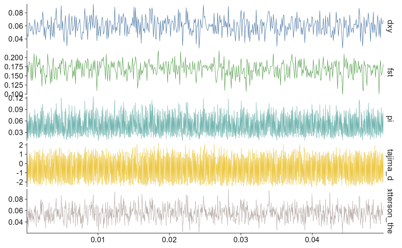

Faceted line plot of population genomics statistics across chr2L. Five statistic panels are stacked vertically for Dxy, FST, pi, Tajima's D, and Watterson's theta. Genomic position in megabases is on the shared x-axis from 1 to 50,000 bases, and each panel has its own statistic value scale.

The same plotting path works for vcftools imports:

plot_stats(vcftools_stats, stat = "all", chr = "chr2L")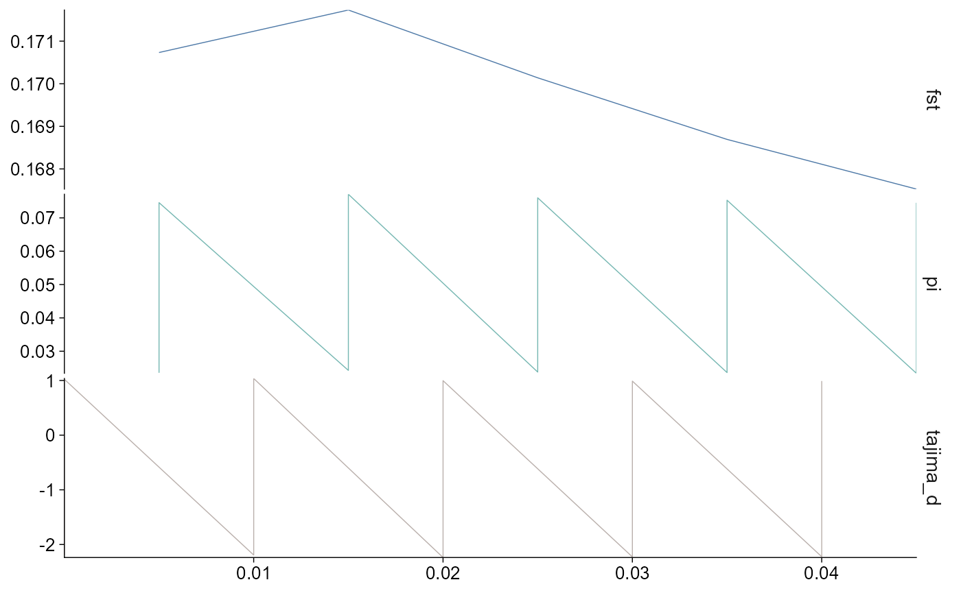

Faceted line plot from vcftools results. FST, pi, and Tajima's D are stacked vertically, genomic position in megabases is on the x-axis, and each panel has its own statistic value scale.

Select statistics and regions

Use stat to choose one or more summaries, chr to select chromosomes, and start / end to focus on windows overlapping a region.

plot_stats(stats, stat = c("fst", "pi"), chr = "chr2L")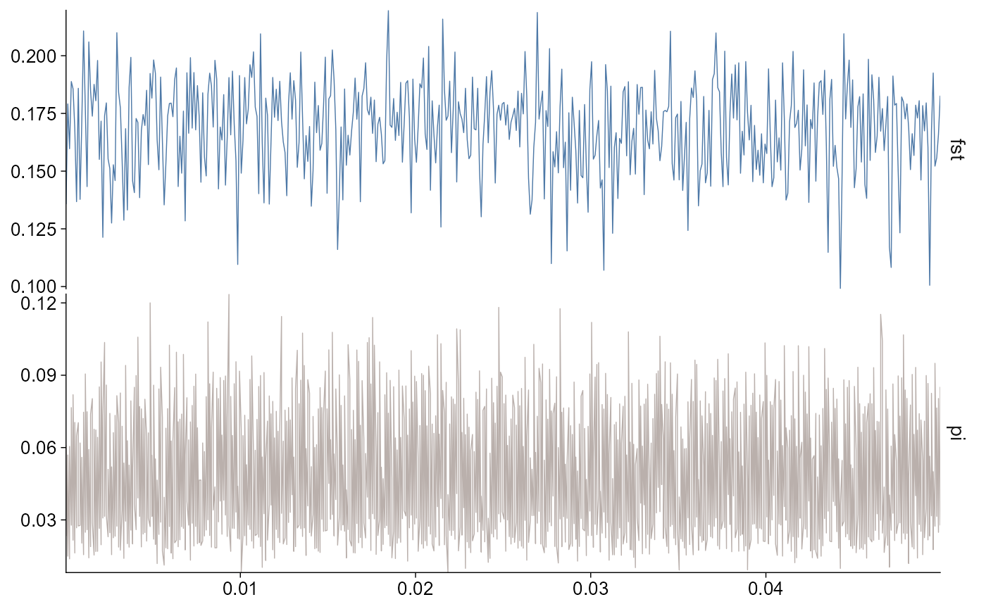

Two-panel line plot. FST and pi are stacked vertically for chromosome chr2L using 100 bp windows, with genomic position in megabases on the shared x-axis and each statistic value on its own y-axis.

plot_stats(stats, chr = "chr2L", start = 1, end = 20000)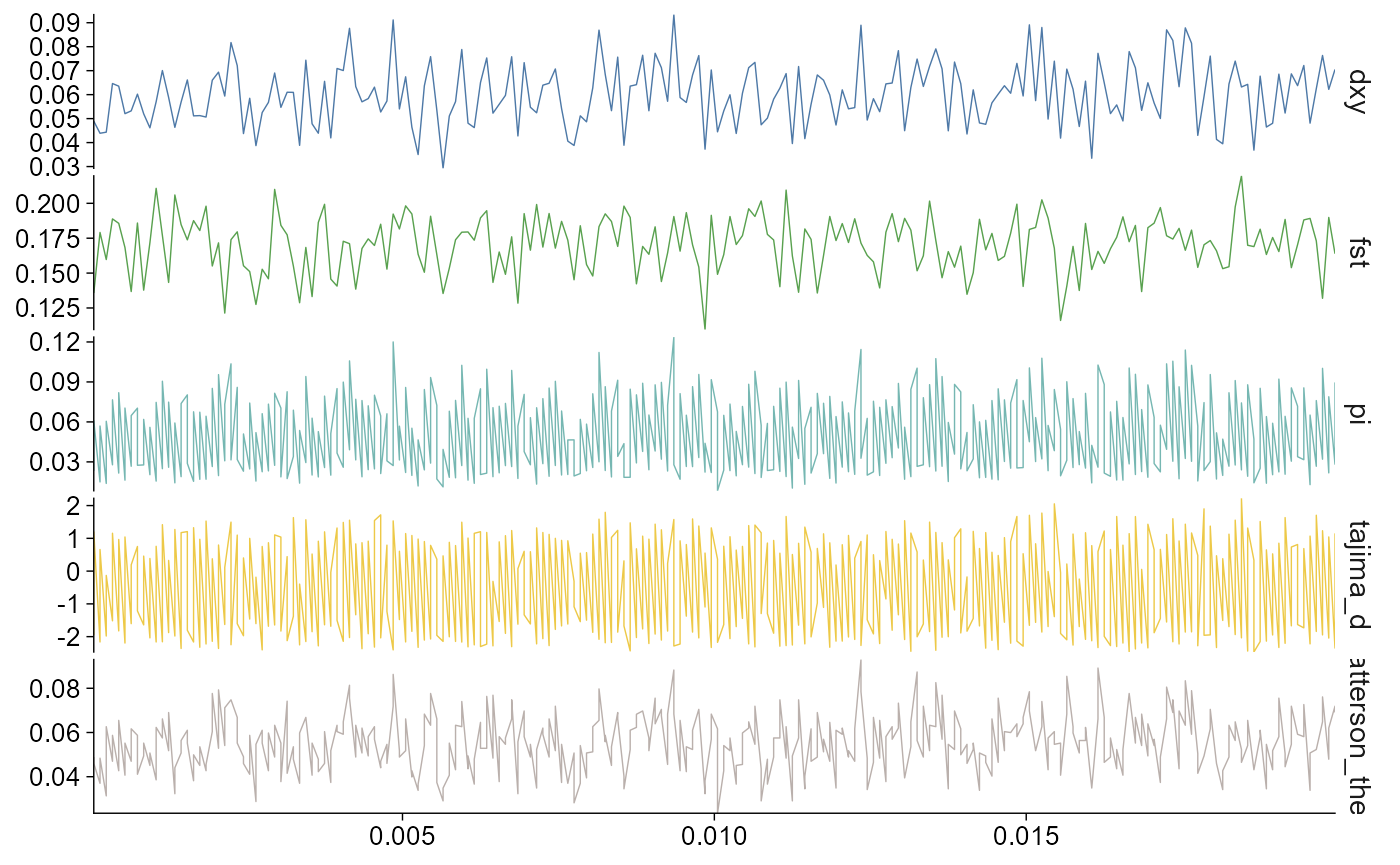

Regional line plot of population genomics statistics. Windows on chromosome chr2L overlapping bases 1 to 20,000 are shown, focusing all statistic panels on the first two-fifths of the bundled 50 kb example region.

Multiple chromosomes can be selected. When more than one chromosome is shown, the default plot uses points to avoid implying continuous genomic distance between chromosomes. The bundled pixy example contains only chr2L, so the multi-chromosome example below uses the vcftools import if multiple chromosomes are present in user data.

plot_stats(stats, chr = c("chr1", "chr2"))

Layered workflow

The layered API follows the same grammar as the other modules:

stats |>
  ggpop() +
  geom_stats(stat = c("fst", "pi"), chr = "chr2L")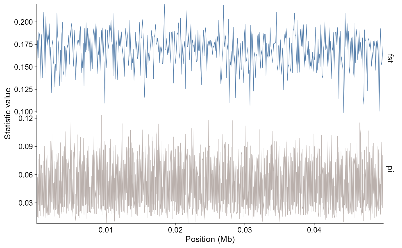

Layered line plot of FST and pi. The ggpop object supplies imported population statistics and geom_stats draws two vertically stacked statistic panels for chromosome chr2L.

The module uses ggpop’s shared theme, font sizing, and discrete palette interfaces. Use palette, base_size, and base_family the same way as the GWAS and PCA modules.