Selective sweep scans • ggPopi

ggpop imports selection scan outputs into a typed ggpop_selection object. The module supports common selscan normalized outputs and XPCLR window tables.

API summary

Task	API	Notes
Import selscan results	`import_selection(dir, type = "selscan")`	Auto-discovers iHS, nSL, iHH12, XP-EHH, and XP-nSL norm files
Import XPCLR windows	`import_selection(dir, type = "xpclr")`	Uses window midpoint as `pos` and keeps `start` / `end`
Direct plot	`plot_selection(data, stat = ..., chr = ...)`	Returns a `ggplot` object
Layered plot	`ggpop(data) + geom_selection(...)`	Tidy ggplot extension path
Region filter	`chr`, `start`, `end`	Keeps points or windows overlapping the region
Plot style	`style = "auto"` / `"single"` / `"manhattan"`	Genome-wide calls default to Manhattan-like; local calls default to single-region
Thresholds	`threshold = 2` or `threshold = 0.95, threshold_type = "quantile"`	Fixed score cutoffs or filtered-data quantiles
Score sign	`value = "signed"` / `"absolute"`	Signed z-score-like views or absolute outlier magnitude

Import selscan results

The bundled selscan example contains normalized iHS, nSL, iHH12, XP-EHH, and XP-nSL outputs. Directory imports auto-discover supported result files.

selscan_dir <- ggpop_extdata("selective_sweep", "selscan")
selscan <- import_selection(selscan_dir, type = "selscan")
class(selscan)
#> [1] "ggpop_selection" "data.frame"
unique(selscan$stat)
#> [1] "ihh12" "ihs"   "nsl"   "xpehh" "xpnsl"

You can also import selected files explicitly. Relative paths are resolved inside dir.

selscan_chr1 <- import_selection(
  selscan_dir,
  ihs = "chr1.ihs.out.100bins.norm",
  nsl = "chr1.nsl.out.100bins.norm",
  xpehh = "chr1.xpehh.out.norm",
  xpnsl = "chr1.xpnsl.out.norm",
  type = "selscan"
)
unique(selscan_chr1$stat)
#> [1] "ihh12" "ihs"   "nsl"   "xpehh" "xpnsl"

Plot scan statistics

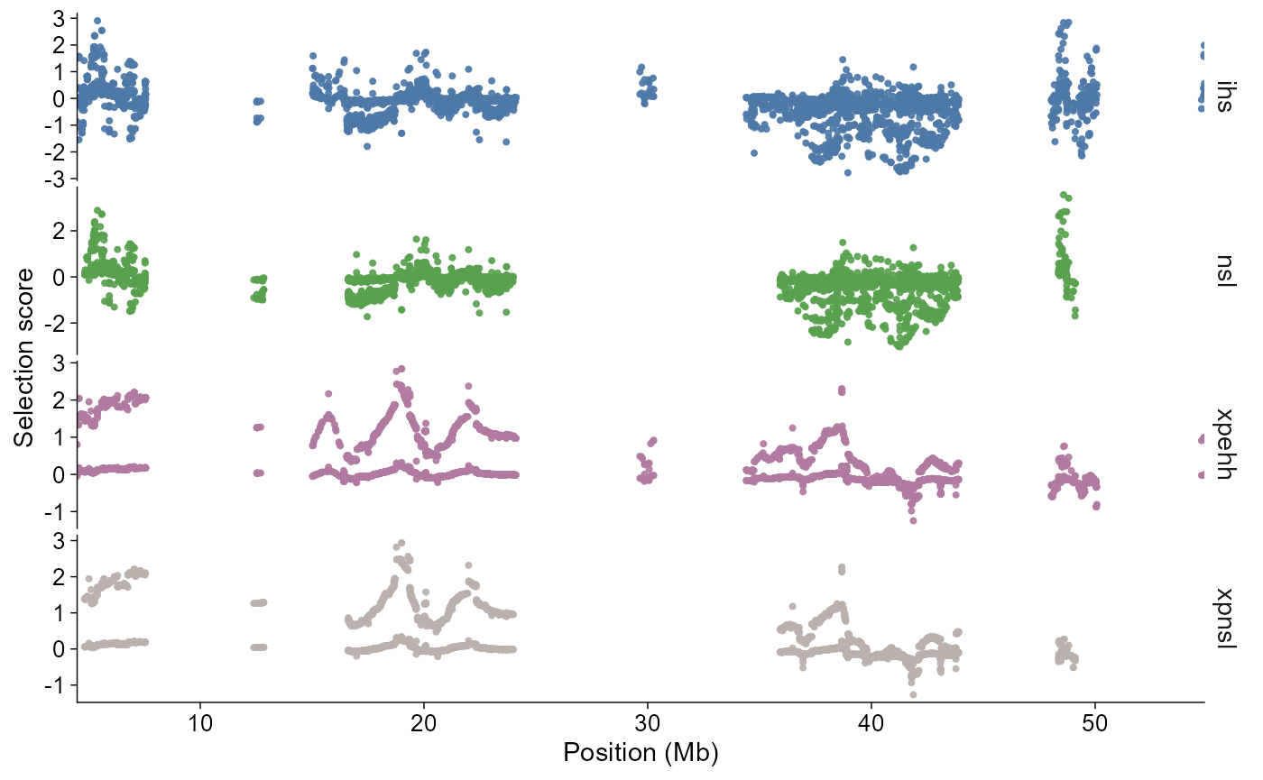
plot_selection() stacks selected statistics vertically and keeps genomic position aligned on the x-axis. Region filters work on points for selscan and on overlapping windows for XPCLR. By default, genome-wide calls use a Manhattan-like chromosome axis. Calls with chr, start, or end use the single-region style, where position is shown directly in megabases.

plot_selection(
  selscan_chr1,
  stat = c("ihs", "nsl", "xpehh", "xpnsl"),
  chr = "1"
)

Faceted scatter plot of four selscan statistics on chromosome 1. iHS, nSL, XP-EHH, and XP-nSL are stacked vertically with genomic position in megabases on the shared x-axis.

The layered API follows the same grammar as the other modules:

selscan_chr1 |>
  ggpop() +
  geom_selection(stat = "ihs", chr = "1", threshold = 2)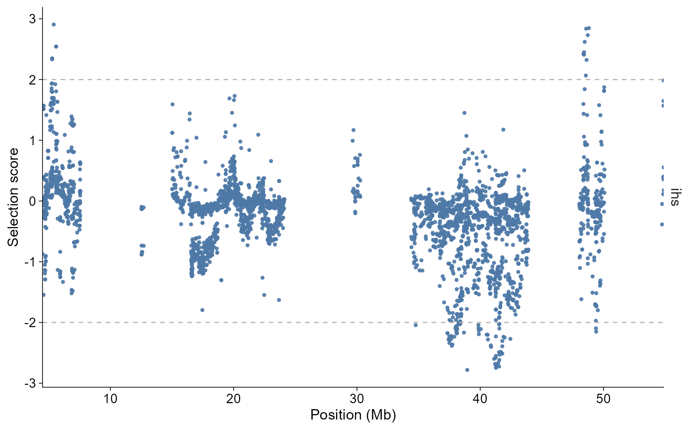

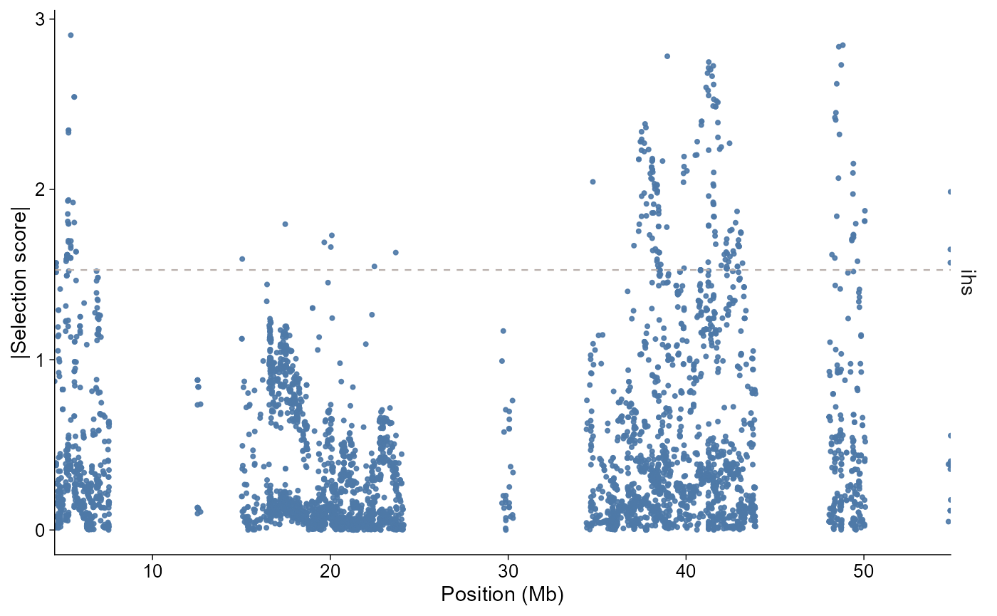
Layered ggplot selection scan. The ggpop object supplies imported selscan data, and geom_selection draws iHS values for chromosome 1 with horizontal threshold lines.

Use value = "absolute" when the direction of the statistic is less important than the magnitude. Quantile thresholds are computed after the statistic, chromosome, and region filters are applied.

plot_selection(
  selscan_chr1,
  stat = "ihs",
  chr = "1",
  value = "absolute",
  threshold = 0.95,
  threshold_type = "quantile"
)

Absolute iHS selection scan on chromosome 1. The y-axis shows absolute selection score magnitude, with a dashed horizontal line at the 95th percentile of the filtered chromosome 1 iHS values.

Manhattan-like genome axis

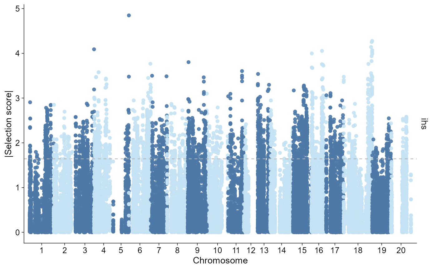
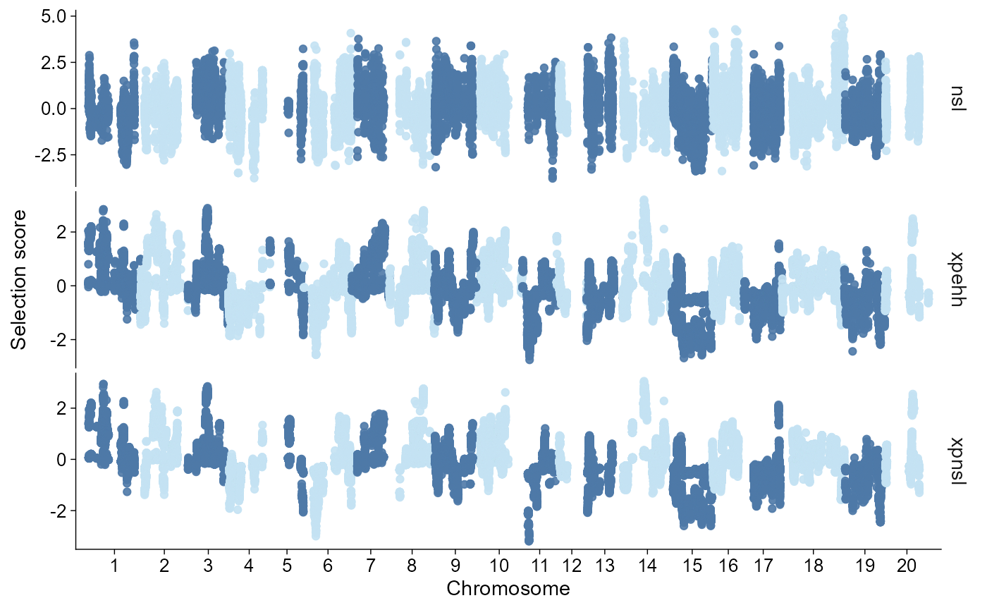
For genome-wide scan summaries, it is often useful to lay chromosomes end to end like a Manhattan plot. Fine-scale structure is compressed, but this view is good for seeing chromosome-scale shifts and scan outliers across the genome.

selscan_selected <- import_selection(
  selscan_dir,
  ihs1 = "chr1.ihs.out.100bins.norm",
  ihs2 = "chr2.ihs.out.100bins.norm",
  ihs3 = "chr3.ihs.out.100bins.norm",
  nsl1 = "chr1.nsl.out.100bins.norm",
  nsl2 = "chr2.nsl.out.100bins.norm",
  nsl3 = "chr3.nsl.out.100bins.norm",
  xpehh1 = "chr1.xpehh.out.norm",
  xpehh2 = "chr2.xpehh.out.norm",
  xpehh3 = "chr3.xpehh.out.norm",
  xpnsl1 = "chr1.xpnsl.out.norm",
  xpnsl2 = "chr2.xpnsl.out.norm",
  xpnsl3 = "chr3.xpnsl.out.norm",
  type = "selscan"
)

finite_scan <- selscan_selected[is.finite(selscan_selected$value), ]

Show absolute iHS on its own scale:

plot_selection(
  finite_scan,
  stat = "ihs",
  style = "manhattan",
  value = "absolute",
  threshold = 0.95,
  threshold_type = "quantile"
)

Manhattan-like selection scan for iHS. Chromosomes 1, 2, and 3 are placed end to end on a continuous genome position axis in megabases, and absolute iHS is plotted as small points coloured by chromosome.

Plot normalized nSL, XP-EHH, and XP-nSL as z-score-like panels:

plot_selection(
  finite_scan,
  stat = c("nsl", "xpehh", "xpnsl"),
  style = "manhattan"
)

Manhattan-like faceted selection scan. nSL, XP-EHH, and XP-nSL are shown in stacked panels over a continuous genome position axis in megabases, with points coloured by chromosome.

Import XPCLR windows

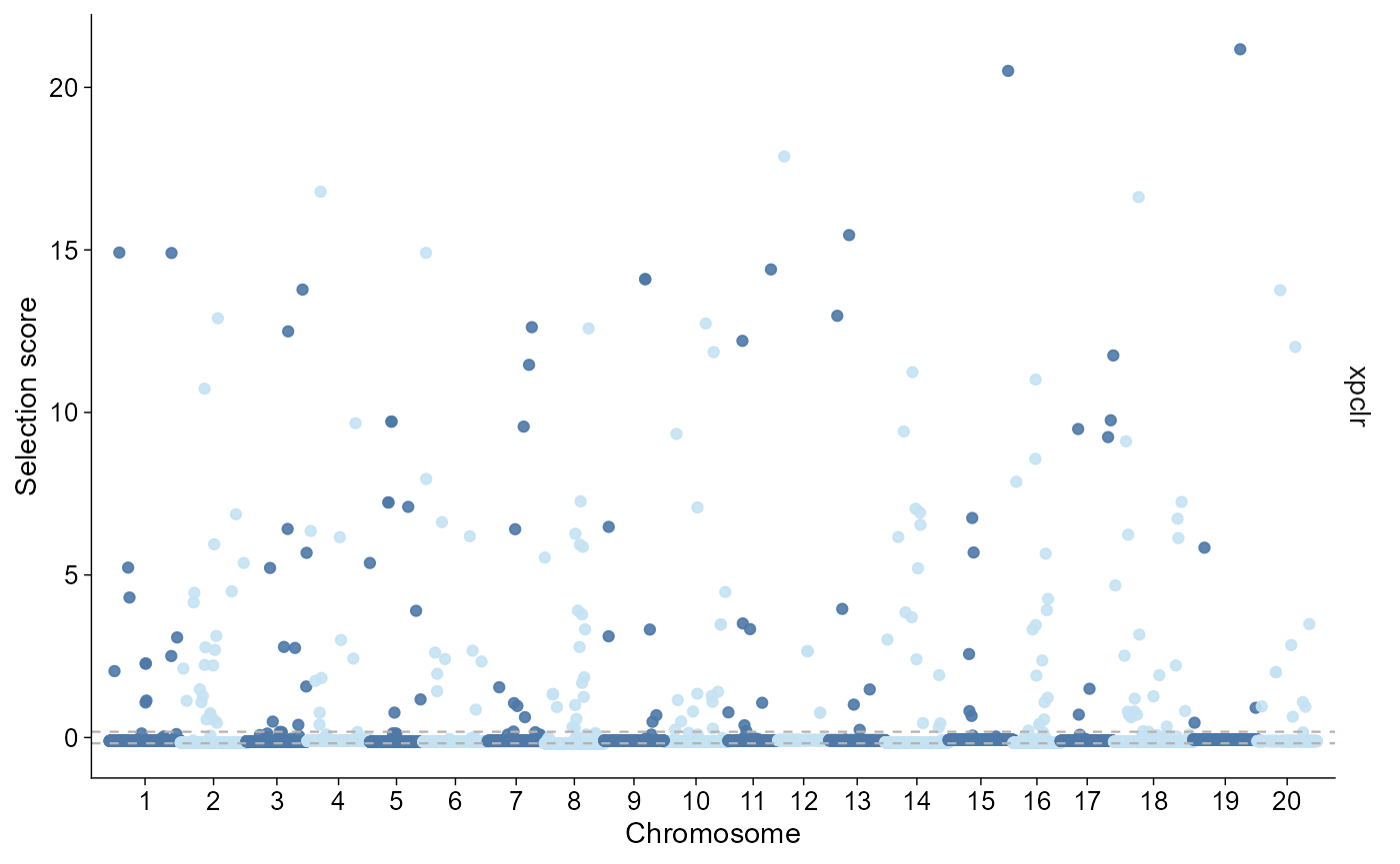
XPCLR outputs are window-based. The importer keeps the original start and end columns, computes pos as the midpoint, and prefers xpclr_norm when it is available.

xpclr_dir <- ggpop_extdata("selective_sweep", "xpclr")
xpclr <- import_selection(xpclr_dir, type = "xpclr")
class(xpclr)
#> [1] "ggpop_selection" "data.frame"
unique(xpclr$stat)
#> [1] "xpclr"
head(xpclr[c("chr", "start", "end", "pos", "value")])
#>                           chr  start   end      pos      value
#> xpclr_allchr_merged.tsv.1   1      1 5e+05 250000.5 -0.1051471
#> xpclr_allchr_merged.tsv.2   1 100001 6e+05 350000.5 -0.1051471
#> xpclr_allchr_merged.tsv.3   1 200001 7e+05 450000.5 -0.1051471
#> xpclr_allchr_merged.tsv.4   1 300001 8e+05 550000.5 -0.1051471
#> xpclr_allchr_merged.tsv.5   1 400001 9e+05 650000.5 -0.1051471
#> xpclr_allchr_merged.tsv.6   1 500001 1e+06 750000.5 -0.1051471

plot_selection(
  xpclr,
  stat = "xpclr",
  style = "manhattan",
  threshold = 0.95,
  threshold_type = "quantile"
)

XPCLR Manhattan-like genome scan. XPCLR window midpoints are placed along a chromosome axis, with normalized XPCLR score on the y-axis and points coloured by chromosome.

Use geom_selection() when the scan should be composed with additional ggplot layers or annotations.