Getting Started with ggPopi • ggPopi

ggPopi is a ggplot2 extension package for population genetics workflows. The package keeps each module in the same tidy shape:

import_*() functions create typed S3 objects.
plot_*() functions return full ggplot objects.
ggpop() + geom_*() build layered ggplot extensions.
Advanced compatibility helpers remain exported for users who need original-package behavior.

The package name is ggPopi; the core layered constructor remains ggpop() for API continuity.

Module API map

Module	Import	Direct plot	ggplot extension path	Advanced / compatibility
GWAS Manhattan	`import_gwas()`	`plot_manha()`	`ggpop() + geom_manha()`	internal fastman-style layout
GWAS Q-Q	`import_gwas()`	`plot_qq()`	`ggpop() + ggPopi::geom_qq()`	internal fastqq-style layout
PCA	`import_pca()` / `compute_pca()`	`plot_pca()`	`ggpop() + geom_pca()`	`compute_pca(method = "flashpca")`
Admixture	`import_admix()`	`plot_admix()`	`ggpop() + geom_admix()`	see compatibility article
Population statistics	`import_stats()`	`plot_stats()`	`ggpop() + geom_stats()`	pixy and vcftools summaries
LD decay	`import_ld_decay()`	`plot_ld_decay()`	`ggpop() + geom_ld_decay()`	PopLDdecay and PLINK summaries
Selective sweeps	`import_selection()`	`plot_selection()`	`ggpop() + geom_selection()`	selscan and XPCLR scans
Introgression	`import_introgression()`	`plot_introgression()`	`ggpop() + geom_introgression()`	Dsuite local/trio statistics, ADMIXTOOLS f-stat tables, and TreeMix summaries
Ne history	`import_ne_history()`	`plot_ne_history()`	`ggpop() + geom_ne_history()`	PSMC, MSMC2, SMC++, and Stairway Plot 2 histories

Core pattern

gwas <- import_gwas(ggpop_extdata("gwas", "gcta.mlma"), type = "gcta")
pca <- import_pca(
  ggpop_extdata("pca", "gcta.eigenvec"),
  type = "gcta",
  eigenval = ggpop_extdata("pca", "gcta.eigenval"),
  pop_group = ggpop_extdata("pop_group.txt")
)
admix <- import_admix(
  ggpop_extdata("admixture"),
  type = "admixture",
  ind = ggpop_extdata("snp", "finalsnp_ld.fam"),
  pop_group = ggpop_extdata("pop_group.txt")
)
stats <- import_stats(
  ggpop_extdata("Population_genomics_statistics", "pixy"),
  type = "pixy"
)
ld_decay <- import_ld_decay(
  ggpop_extdata("ld_decay", "poplddcay"),
  type = "poplddecay"
)
ld_grouped <- import_ld_decay(
  ggpop_extdata("ld_decay", "poplddcay"),
  type = "poplddecay"
)
selscan_chr1 <- import_selection(
  ggpop_extdata("selective_sweep", "selscan"),
  ihs = "chr1.ihs.out.100bins.norm",
  nsl = "chr1.nsl.out.100bins.norm",
  xpehh = "chr1.xpehh.out.norm",
  xpnsl = "chr1.xpnsl.out.norm",
  type = "selscan"
)
introgression <- import_introgression(
  ggpop_extdata("introgression", "Dsuite", "PopB_PopC_PopA_localFstats_run1_100_50.txt"),
  type = "dsuite_dinvestigate"
)
ne_history <- import_demographic_history(
  ggpop_extdata("ne_history", "SMC++", "model.csv"),
  type = "smcpp",
  mutation_rate = 1.2e-8,
  generation_time = 5
)

Each importer returns a typed object:

class(gwas)
#> [1] "ggpop_gwas" "data.frame"
class(pca)
#> [1] "ggpop_pca"  "data.frame"
class(admix)
#> [1] "ggpop_admix" "data.frame"
class(stats)
#> [1] "ggpop_stats" "data.frame"
class(ld_decay)
#> [1] "ggpop_ld_decay" "data.frame"
class(ld_grouped)
#> [1] "ggpop_ld_decay" "data.frame"
class(selscan_chr1)
#> [1] "ggpop_selection" "data.frame"
class(introgression)
#> [1] "ggpop_introgression" "data.frame"
class(ne_history)
#> [1] "ggpop_ne_history" "data.frame"

Tidy plotting style

Every module has two user-facing plotting paths. Use the direct plot_*() function when you want the reference plot immediately, or use ggpop() plus the module geom_*() when you want to compose with other ggplot layers.

The direct path:

gwas |>
  plot_manha()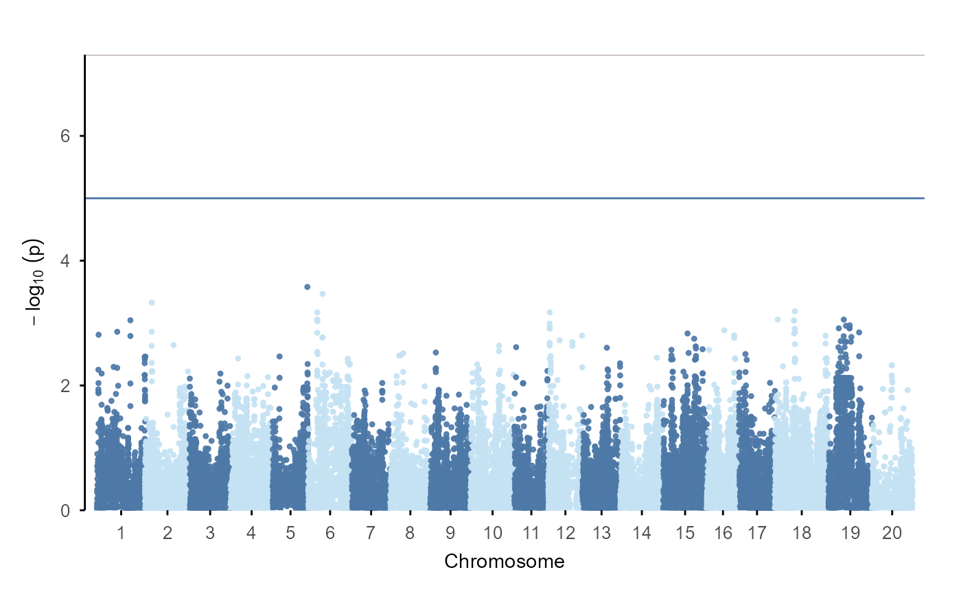

Manhattan plot. Chromosomes are arranged along the x-axis and minus log10 p-values are on the y-axis. Points form chromosome-specific bands with horizontal reference lines marking suggestive and genome-wide significance thresholds.

The ggplot extension path:

gwas |>
  ggpop() +
  geom_manha()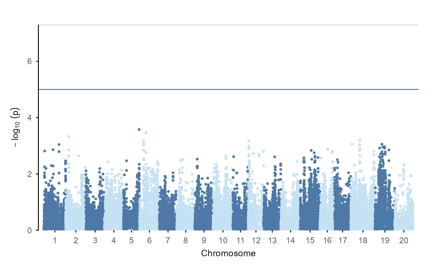

Manhattan plot from the layered ggplot extension path. Chromosomes are arranged along the x-axis and minus log10 p-values are on the y-axis, matching the direct plot_manha visual style.

The same pattern applies across modules:

gwas |> ggpop() + ggPopi::geom_qq()

Q-Q scatter plot. Expected minus log10 p-values are on the x-axis and observed minus log10 p-values are on the y-axis, with points compared against a diagonal reference line.

pca |> ggpop() + geom_pca()

Scatter chart. Principal component 1 is on the x-axis and principal component 2 is on the y-axis, with point colour encoding population groups.

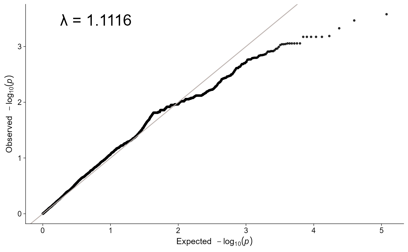
admix |> ggpop() + geom_admix(k = 3, order_group = TRUE)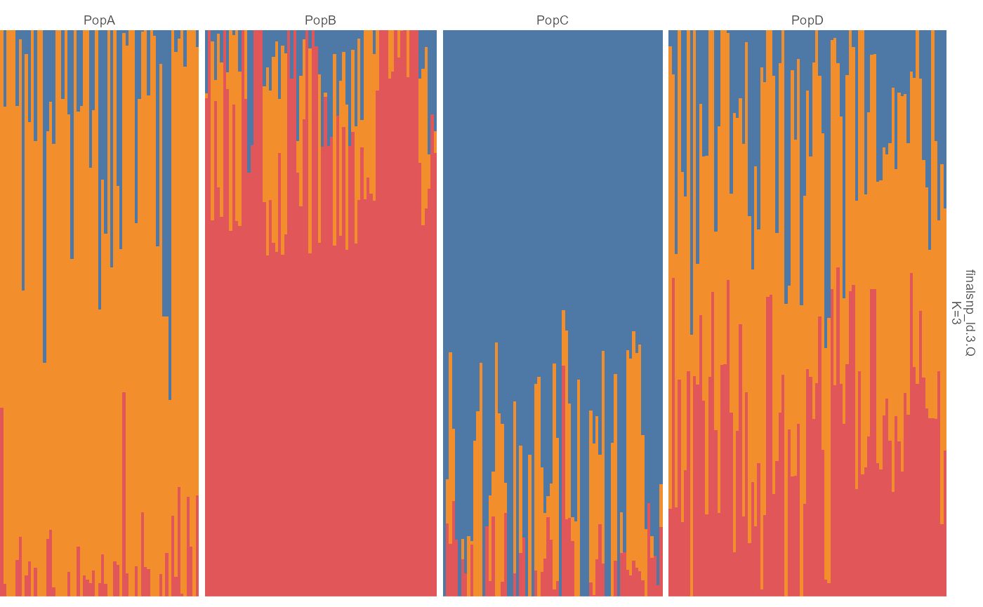

Stacked bar chart. Individuals are arranged along the x-axis and ancestry proportions are stacked within each bar for K equals 3.

Population groups and discrete colours

Population grouping uses a simple two-column file:

head(import_pop_group(ggpop_extdata("pop_group.txt")))
#>   sample_id  pop
#> 1      P001 PopC
#> 2      P004 PopB
#> 3      P006 PopC
#> 4      P009 PopA
#> 5      P010 PopB
#> 6      P012 PopB

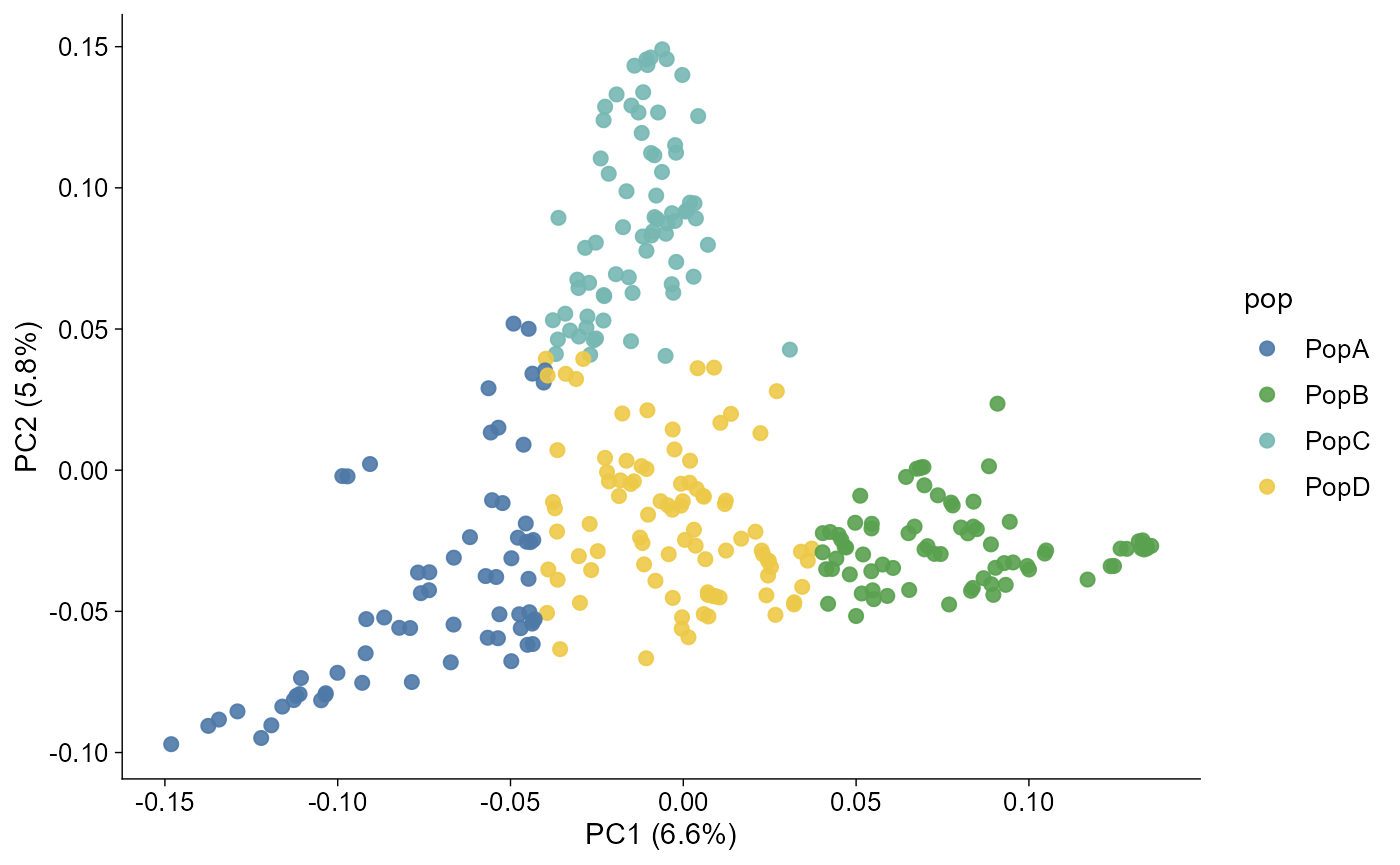
The same file drives PCA colours and admixture group labels:

pca |> plot_pca()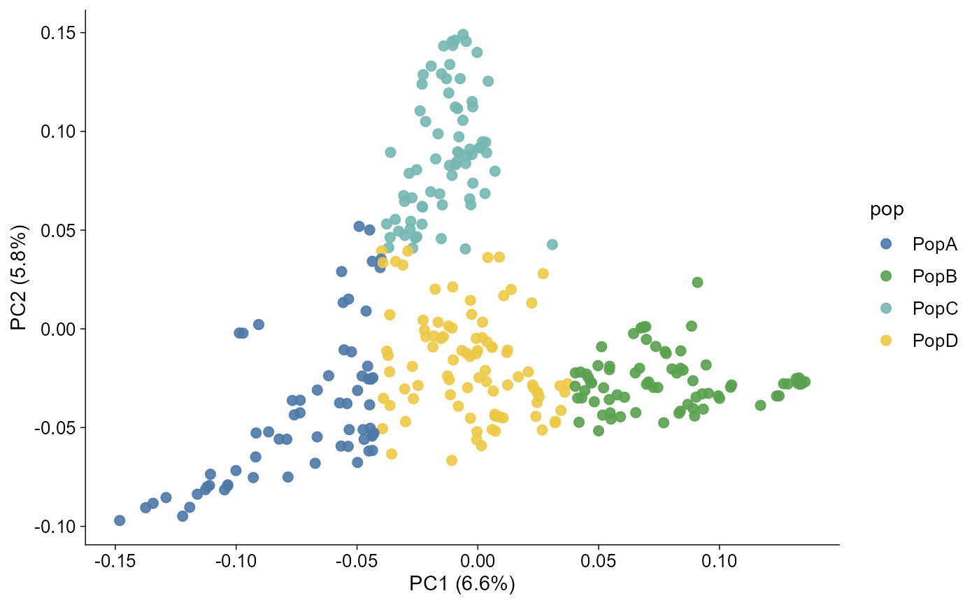

Scatter chart. Principal component 1 is on the x-axis and principal component 2 is on the y-axis, with point colour encoding imported population groups.

admix |> plot_admix(k = 3, order_group = TRUE, show_group_labels = TRUE)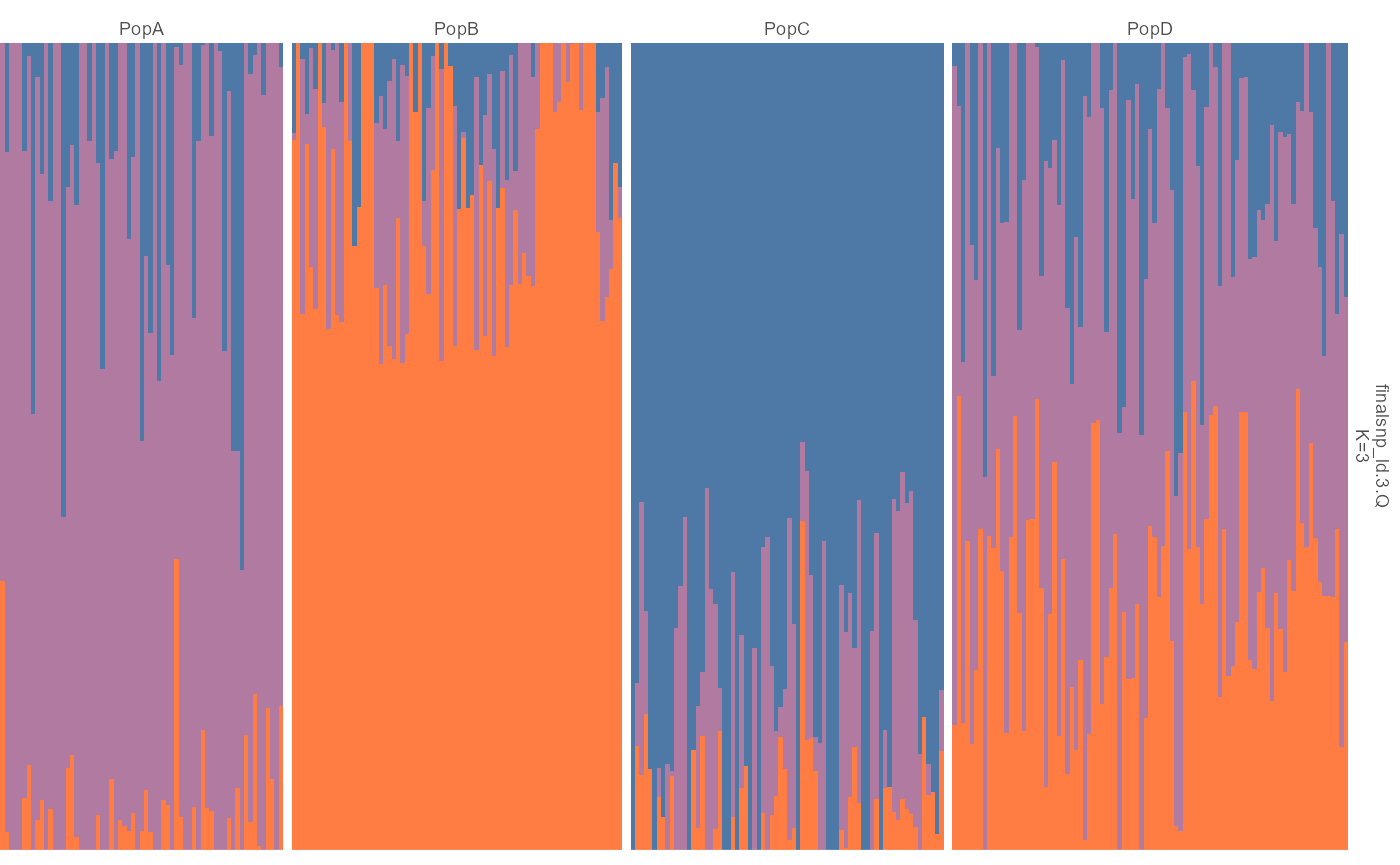

Stacked bar chart. Individuals are arranged along the x-axis and ancestry proportions are stacked within each bar, with population group labels used for ordering.

All categorical colours use a unified discrete palette entry:

ggpop_palette(4, "population")
#> [1] "#4E79A7" "#59A14F" "#76B7B2" "#EDC948"
ggpop_palette(8, "admixture")
#> [1] "#4E79A7" "#F28E2B" "#E15759" "#76B7B2" "#EDC948" "#9C755F"
#> [7] "#2F4B7C" "#FF7C43"

Population statistics

The statistics module uses the same tidy pattern for windowed summaries from pixy or vcftools outputs:

stats |>
  plot_stats(stat = "all", chr = "chr2L")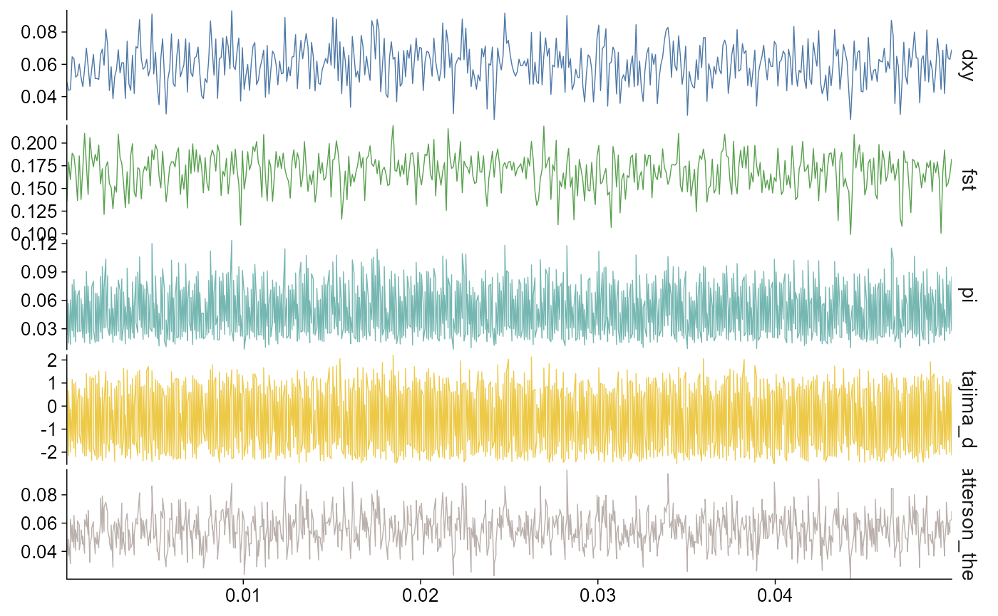

Faceted line plot of population genomics statistics on chr2L. Dxy, FST, pi, Tajima's D, and Watterson's theta are stacked vertically, genomic position in megabases is on the shared x-axis, and each panel uses its own statistic value scale.

The layered path filters facets to the requested statistics:

stats |>
  ggpop() +
  geom_stats(stat = c("fst", "pi"), chr = "chr2L")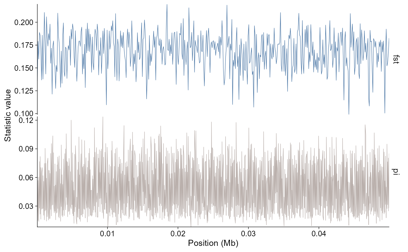

Layered two-panel line plot of population genomics statistics. The ggpop object supplies imported pixy statistics and geom_stats draws only the selected FST and pi facets for chr2L.

LD decay

LD decay summaries use the same direct and layered plotting shape. PopLDdecay *.stat.gz files are imported directly, while PLINK pairwise LD files can be summarized into distance bins. Population labels follow the package-wide pop_group.txt convention when file labels need to be mapped to groups. Point and line styles keep the imported summary rows; style = "fit" draws population-level fitted curves.

ld_grouped |>
  plot_ld_decay(style = "point")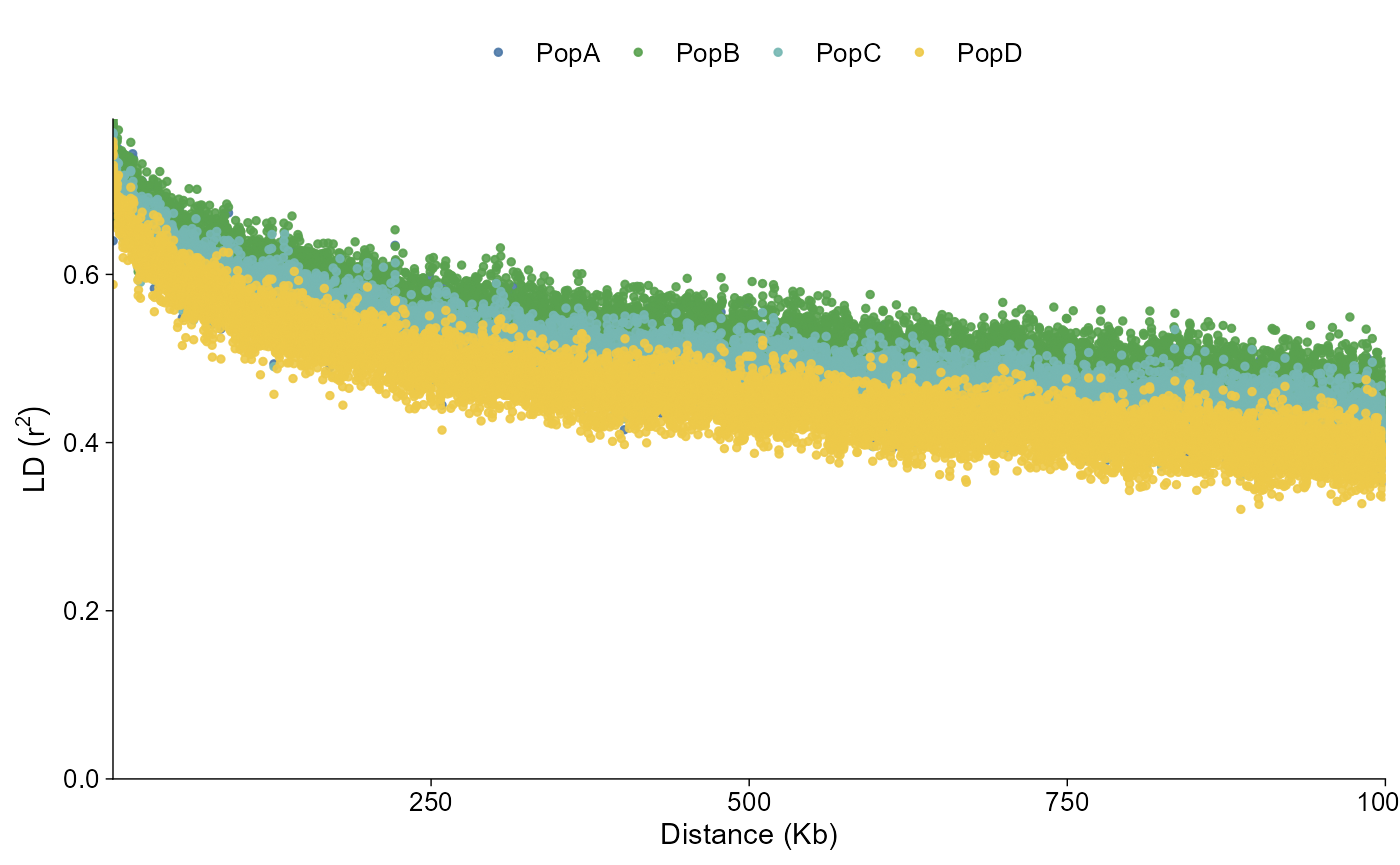

LD decay point plot. Pairwise distance in kilobases is on the x-axis and mean LD r squared is on the y-axis, with points coloured by population label.

The same data can be drawn as a connected curve:

ld_grouped |>
  plot_ld_decay(style = "line")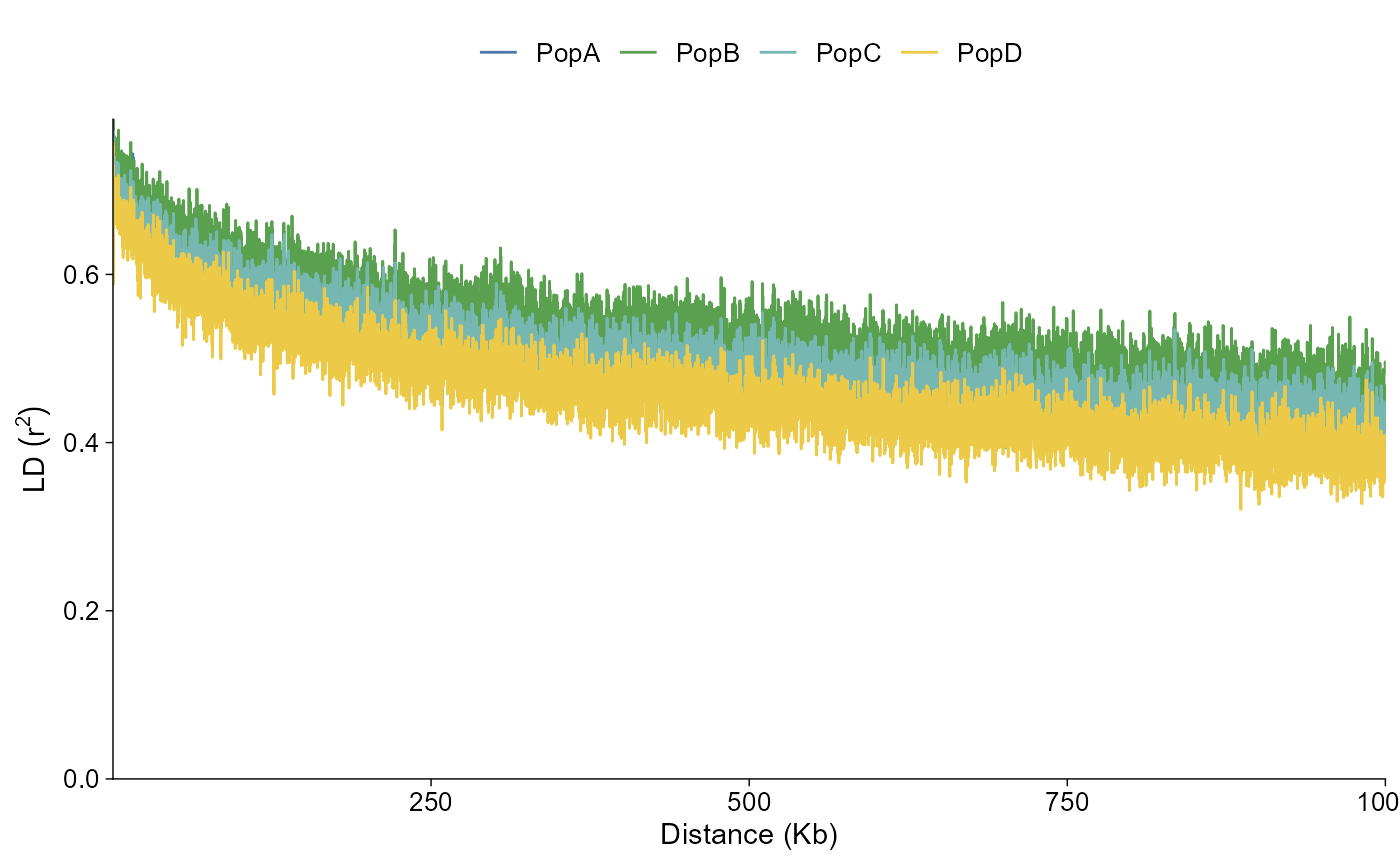

LD decay line plot. Pairwise distance in kilobases is on the x-axis and mean LD r squared is on the y-axis, with a continuous curve showing the decay pattern.

Or as population-level fitted curves:

ld_grouped |>
  plot_ld_decay(style = "fit")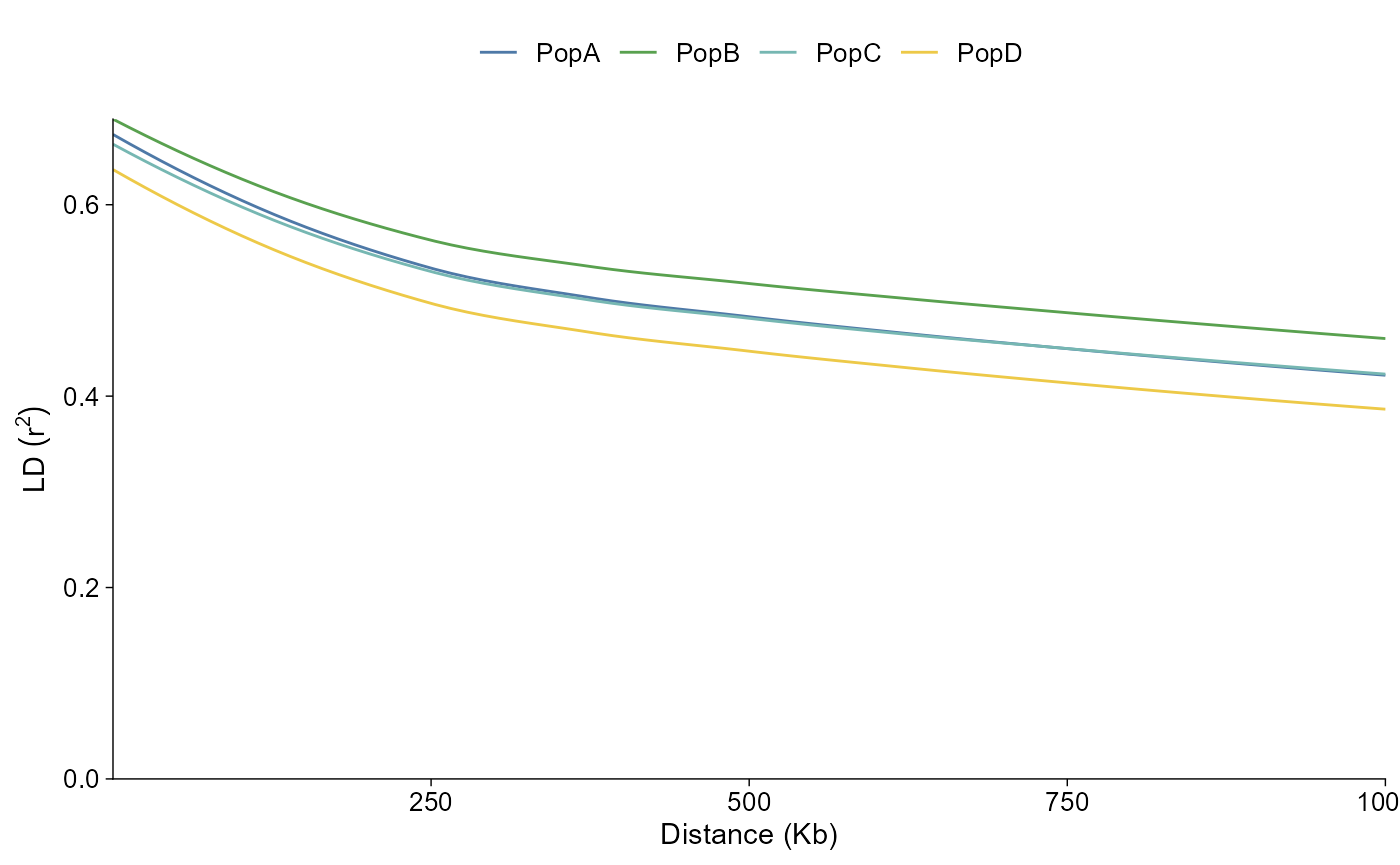

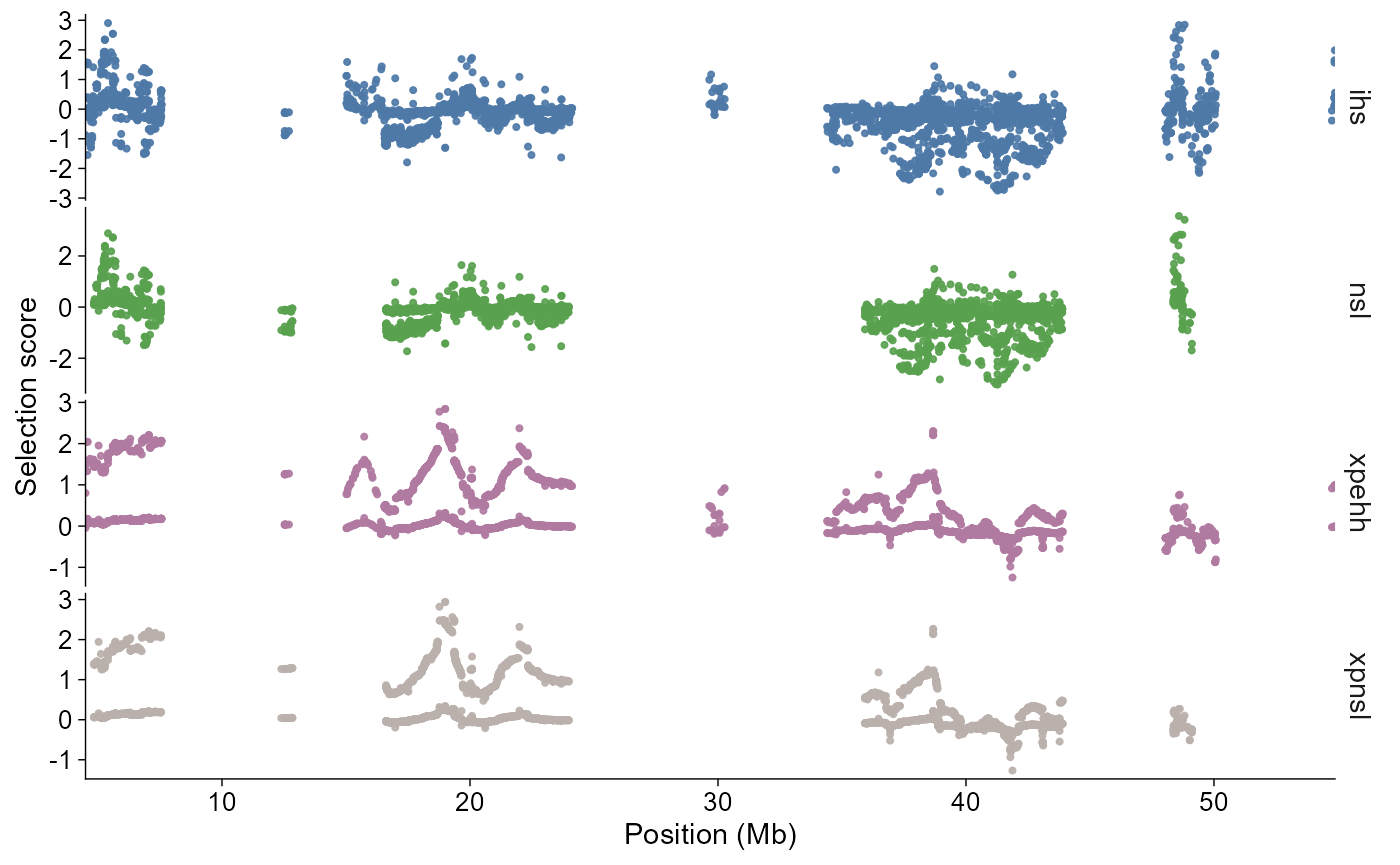
LD decay fitted line plot. Pairwise distance in kilobases is on the x-axis and mean LD r squared is on the y-axis, with fitted curves coloured by population label.

Selective sweep scans

Selection scan outputs use the same direct and layered plotting shape. The direct plot can show signed values or absolute score magnitude, and thresholds can be fixed values or filtered-data quantiles. Genome-wide calls default to a Manhattan-like chromosome axis; calls with chr, start, or end default to a single-region view.

selscan_chr1 |>
  plot_selection(
    stat = c("ihs", "nsl", "xpehh", "xpnsl"),
    chr = "1"
  )

Faceted selection scan on chromosome 1. iHS, nSL, XP-EHH, and XP-nSL are stacked vertically with genomic position in megabases on the x-axis.

Introgression

Introgression summaries use the same direct and layered plotting shape. Windowed Dsuite localFstats/Dinvestigate outputs default to chromosome-wise window points on a Manhattan-like genome axis. Dsuite BBAA/Dmin trio summaries default to P2-by-P3 matrix/raster views, with ordered forest/lollipop summaries available through style = "trio". ADMIXTOOLS qpdstat, f3, and f4ratio outputs are imported as trio statistic summaries and drawn as forest/lollipop panels with standard-error bars when available. TreeMix internal edge/treeout outputs are shown as lightweight graph summaries; matching vertices files preserve the TreeMix drift-coordinate layout.

The bundled example below is a compact Dsuite localFstats window table. It is meant for plotting examples; production analyses should import the real Dsuite, ADMIXTOOLS, or TreeMix output files.

introgression |>
  plot_introgression(stat = c("D", "fdM"))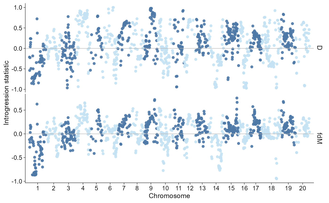

Window introgression plot. D and fdM statistics are shown as chromosome-wise Manhattan-like points in stacked panels over the genome.

The layered path follows the same grammar:

introgression |>
  ggpop() +
  geom_introgression(stat = "D")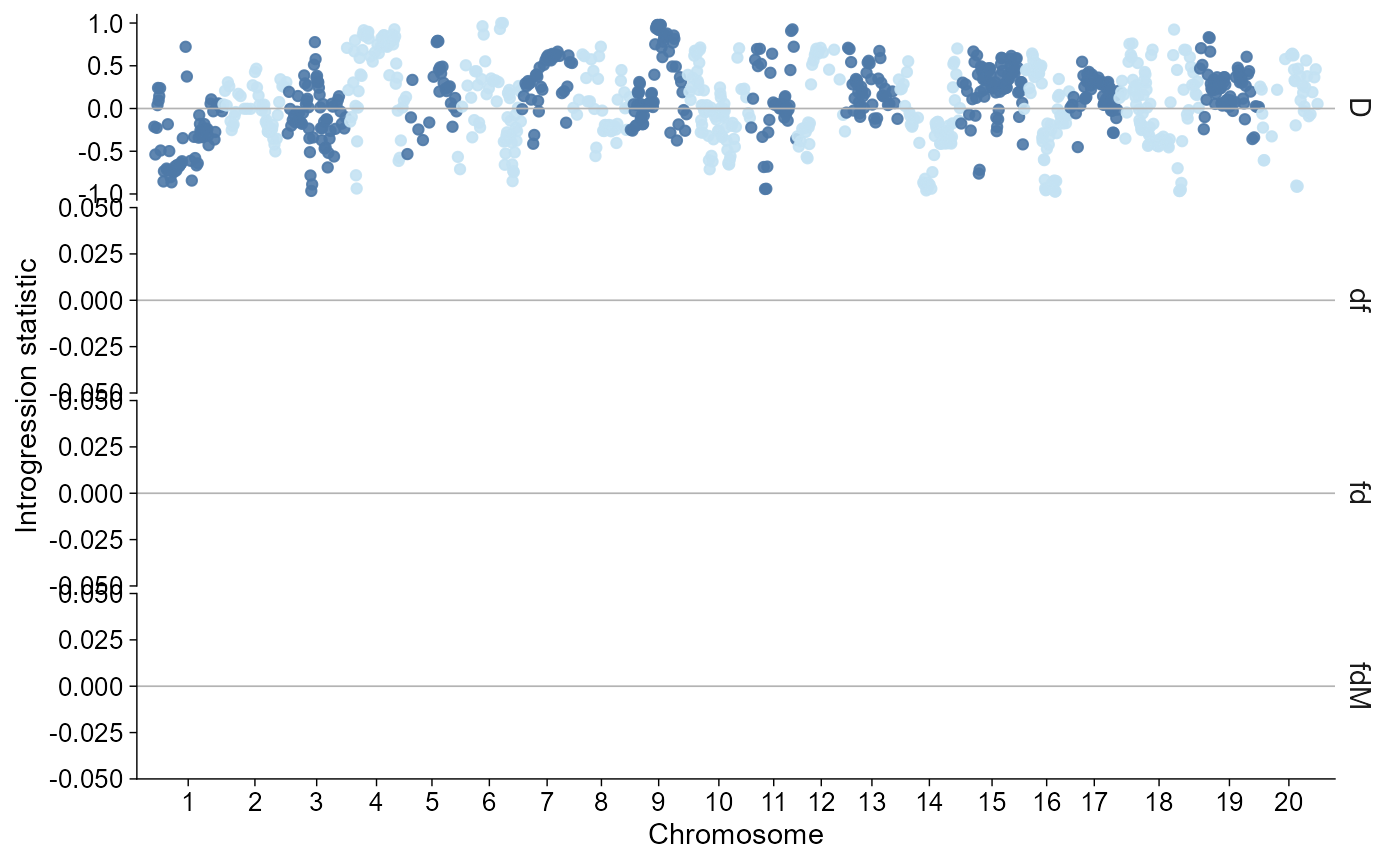

Layered introgression plot using ggpop plus geom_introgression. D statistic windows are drawn as chromosome-wise Manhattan-like points over the genome.

Ne history

Effective population size histories from PSMC, MSMC2, SMC++, and Stairway Plot 2 use the same direct and layered plotting shape. SMC++ histories are drawn as curves, while PSMC, MSMC2, and Stairway Plot 2 interval histories default to step curves. Time and Ne axes are log-scaled by default.

import_demographic_history(), plot_demographic_history(), and geom_demographic_history() are aliases for the same API. The bundled SMC++ example follows the Acropora-style CSV shape and uses pop_group.txt population labels (PopA-PopD) with biologically plausible bottleneck and recovery trajectories plus bootstrap paths.

Raw VCF and pop_group.txt metadata are inputs to external demographic inference workflows. ggPopi imports the resulting PSMC, MSMC2, SMC++, or Stairway Plot 2 outputs; it does not infer Ne histories directly from VCF.

ne_history |>
  plot_demographic_history()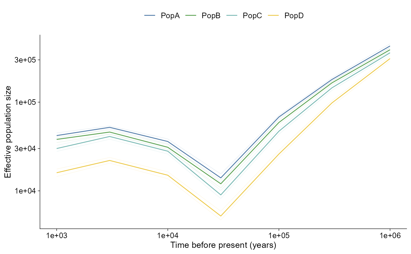

Effective population size history plot. Time before present is on the x-axis and effective population size is on the y-axis, with separate curves for four populations and faint bootstrap trajectories behind the main curves.

The layered path follows the same grammar:

ne_history |>
  ggpop() +
  geom_demographic_history()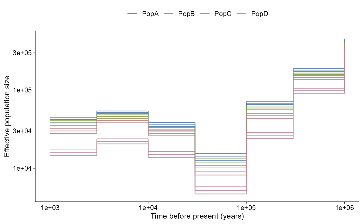

Layered demographic history plot using ggpop plus geom_demographic_history. Population-specific SMC++ curves are drawn on log-scaled time and Ne axes with bootstrap trajectories behind the main curves.

What to use

Use plot_manha() and ggpop() + geom_manha() for Manhattan plots.
Use plot_qq() and ggpop() + ggPopi::geom_qq() for Q-Q plots.
Use plot_pca() and ggpop() + geom_pca() for PCA plots.
Use plot_admix() and ggpop() + geom_admix() for admixture plots.
Use plot_stats() and ggpop() + geom_stats() for windowed population statistics.
Use plot_ld_decay() and ggpop() + geom_ld_decay() for LD decay summaries.
Use plot_selection() and ggpop() + geom_selection() for selective sweep scans.
Use plot_introgression() and ggpop() + geom_introgression() for introgression summaries.
Use plot_ne_history() / plot_demographic_history() and ggpop() + geom_ne_history() / geom_demographic_history() for effective population size histories.
Treat the direct plot_*() functions as the reference style; geom_*() is the same look inside a ggplot composition.
Use the compatibility article only when you need original pophelper workflows.