LD decay

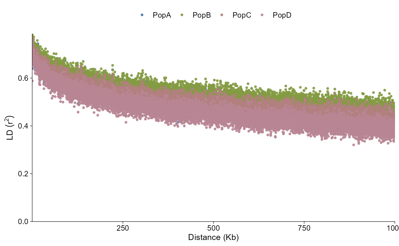
ggpop imports LD decay summaries into a typed ggpop_ld_decay object. The module supports PopLDdecay *.stat.gz summaries and PLINK pairwise LD tables summarized into distance bins. PopLDdecay summaries can be left as-is or collapsed again with method = "MeanBin", MedianBin, or PercentileBin.

API summary

Task	API	Notes
Import PopLDdecay summaries	import_ld_decay(dir, type = "poplddecay")	Reads *.stat.gz and *.bin.gz files directly
Import PLINK LD pairs	import_ld_decay(file, type = "plink")	Summarizes pairwise LD into distance bins
Direct plot	plot_ld_decay(data, style = "point")	Returns a ggplot object
Layered plot	ggpop(data) + geom_ld_decay(...)	Tidy ggplot extension path
Plot style	style = "point" / "line" / "fit"	Raw summary points, connected summary lines, or fitted curves
Measure view	measure = "r2" / "D" / "both"	D' needs PopLDdecay D output
Population labels	pop_group	Uses the package-wide two-column sample pop file

Import PopLDdecay results

The bundled example contains one PopLDdecay *.stat.gz result per population. importer standardizes Dist to dist, Mean_r^2 to r2, and NumberPairs to n_pairs.

ld_dir <- ggpop_extdata("ld_decay", "poplddcay")
ld_decay <- import_ld_decay(ld_dir, type = "poplddecay")
class(ld_decay)
#> [1] "ggpop_ld_decay" "data.frame"
head(ld_decay)
#>                           dist dist_kb        r2 d_prime   sum_r2
#> PopA\rPopA.stat.gz\r10\r0   10    0.01 0.7666593      NA 1687.417
#> PopA\rPopA.stat.gz\r10\r1   20    0.02 0.7609297      NA 2447.911
#> PopA\rPopA.stat.gz\r10\r2   30    0.03 0.7585424      NA 2059.443
#> PopA\rPopA.stat.gz\r10\r3   40    0.04 0.7613730      NA 1764.863
#> PopA\rPopA.stat.gz\r10\r4   50    0.05 0.7546858      NA 1353.152
#> PopA\rPopA.stat.gz\r10\r5   60    0.06 0.7595983      NA 1078.630
#>                           sum_d_prime n_pairs  pop sample_id
#> PopA\rPopA.stat.gz\r10\r0          NA    2201 PopA      PopA
#> PopA\rPopA.stat.gz\r10\r1          NA    3217 PopA      PopA
#> PopA\rPopA.stat.gz\r10\r2          NA    2715 PopA      PopA
#> PopA\rPopA.stat.gz\r10\r3          NA    2318 PopA      PopA
#> PopA\rPopA.stat.gz\r10\r4          NA    1793 PopA      PopA
#> PopA\rPopA.stat.gz\r10\r5          NA    1420 PopA      PopA
#>                                   file ld_method     source .group
#> PopA\rPopA.stat.gz\r10\r0 PopA.stat.gz   MeanBin poplddecay   PopA
#> PopA\rPopA.stat.gz\r10\r1 PopA.stat.gz   MeanBin poplddecay   PopA
#> PopA\rPopA.stat.gz\r10\r2 PopA.stat.gz   MeanBin poplddecay   PopA
#> PopA\rPopA.stat.gz\r10\r3 PopA.stat.gz   MeanBin poplddecay   PopA
#> PopA\rPopA.stat.gz\r10\r4 PopA.stat.gz   MeanBin poplddecay   PopA
#> PopA\rPopA.stat.gz\r10\r5 PopA.stat.gz   MeanBin poplddecay   PopA

Population grouping follows the same pop_group.txt convention used by PCA and admixture. The LD decay file label is stored as sample_id; if a matching sample appears in pop_group, the corresponding pop value is used for colouring. The point and line styles keep the imported summary rows; fit draws population-level fitted curves after mapping sample labels to groups.

The importer also accepts a single file path, and the method argument can be used to re-bin PopLDdecay summaries with the same mean-bin, median, or percentile behavior used by the legacy plotting scripts.

ld_group_dir <- ggpop_extdata("ld_decay", "poplddcay")
ld_grouped <- import_ld_decay(
  ld_group_dir,
  type = "poplddecay"
)
unique(ld_grouped$pop)
#> [1] "PopA" "PopB" "PopC" "PopD"

PLINK pairwise LD tables can be imported the same way. A single .ld file draws one population, while importing the directory keeps one curve per population file.

plink_ld <- import_ld_decay(
  ggpop_extdata("ld_decay", "plink_ld"),
  type = "plink",
  bin_size = 200
)
unique(plink_ld$pop)
#> [1] "PopA" "PopB" "PopC"

Point style

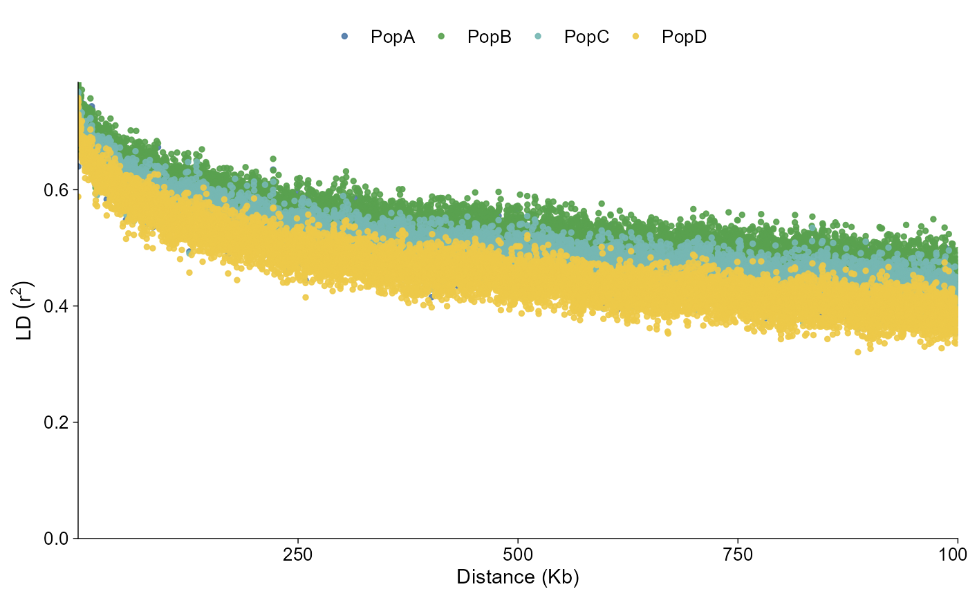
The point style follows the common LD summary plot: pairwise distance in Kb on the x-axis and mean LD $r^2$ on the y-axis, with population labels mapped to colour.

plot_ld_decay(
  ld_grouped,
  style = "point"
)

Line style

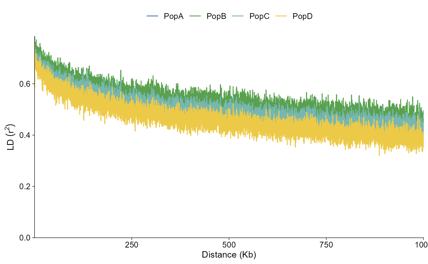
The line style uses the same data and population colour mapping, but draws a continuous decay curve.

plot_ld_decay(
  ld_grouped,
  style = "line"
)

Fitted line style

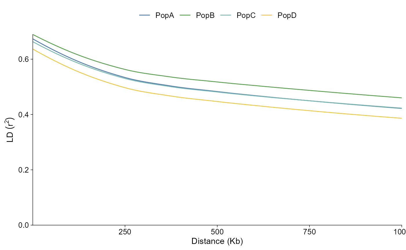
Use style = "fit" when you want a smoothed population-level decay curve.

plot_ld_decay(
  ld_grouped,
  style = "fit"
)

Layered path

Use ggpop() plus geom_ld_decay() when composing with other ggplot layers.

ld_grouped |>
  ggpop() +
  geom_ld_decay(style = "point")