Introgression

ggPopi imports common introgression summaries into a typed ggpop_introgression object. The module is intentionally split by result semantics:

• Dsuite localFstats / Dinvestigate outputs are genomic window scans.
• Dsuite BBAA / Dmin outputs are trio-level D-statistic summaries.
• ADMIXTOOLS qpdstat, f3, and f4ratio outputs are trio statistic tables, not graph edges.
• TreeMix internal *.edges.gz / *.treeout.gz files are imported as a lightweight graph summary. Full TreeMix tree-layout and residual heatmap views belong to a dedicated TreeMix plotting layer.

API summary

Task	API	Notes
Import Dsuite global trio results	import_introgression(file, type = "dsuite_dtrios")	BBAA, Dmin, and similar Dsuite trio tables
Import Dsuite local windows	import_introgression(file, type = "dsuite_dinvestigate")	D, fd, fdM, and df window statistics
Import ADMIXTOOLS statistics	import_introgression(file, type = "admixtools")	qpdstat, f3, and f4ratio CSV/table outputs
Import TreeMix summaries	import_introgression(file, type = "treemix")	Lightweight tree/migration edge summaries
Direct plot	plot_introgression(data, stat = ...)	Returns a ggplot object
Layered plot	ggpop(data) + geom_introgression(...)	Tidy ggplot extension path

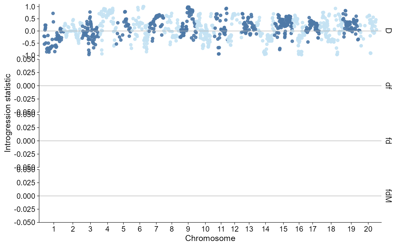
Dsuite Window Scans

Dsuite Dinvestigate / localFstats files are imported in long form, with one row per statistic per genomic window. Genome-wide calls default to a chromosome-wise Manhattan-like window plot, a common pattern in population genomics scripts for D, fd, fdM, and df.

dsuite_windows <- import_introgression(
  ggpop_extdata("introgression", "Dsuite", "PopB_PopC_PopA_localFstats_run1_100_50.txt"),
  type = "dsuite_dinvestigate"
)
class(dsuite_windows)
#> [1] "ggpop_introgression" "data.frame"
unique(dsuite_windows$stat)
#> [1] "D"   "fd"  "fdM" "df"

plot_introgression(dsuite_windows, stat = c("D", "fdM"))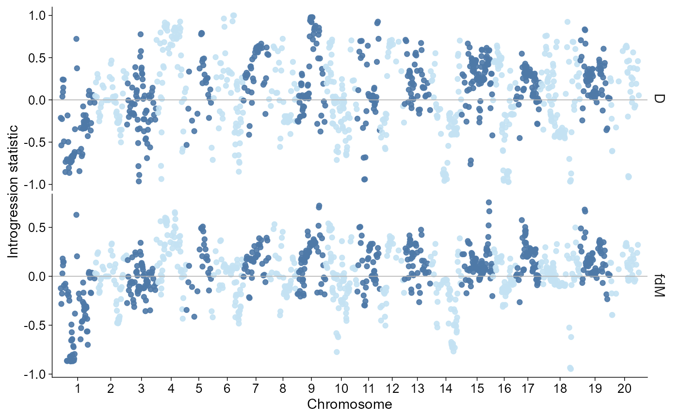

When a chromosome or region is supplied, the direct plot uses a local position axis in megabases and draws a point-and-line trace.

plot_introgression(dsuite_windows, stat = "D", chr = "1")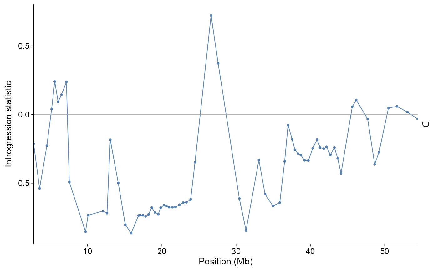

Dsuite Trio Summaries

Dsuite global BBAA / Dmin outputs are imported as trio-level D statistics. The bundled trio table is a biologically structured toy example with highland, lowland, and hybrid populations. The default plot is a Dsuite-style P2 x P3 matrix: population pairs define the tile grid, D statistic defines the diverging fill, and significant cells are outlined without changing the colour scale. If repeated rows share the same P2/P3 combination, the matrix keeps the row with the largest absolute D value and preserves its sign, so strong negative signals remain visible after aggregation. Population labels are cleaned for display only, so names such as Highland_East are plotted as Highland East while the imported data keeps the original identifiers.

dsuite_bbaa <- import_introgression(
  ggpop_extdata("introgression", "Dsuite", "dsuite_results_BBAA.txt"),
  type = "dsuite_dtrios"
)
plot_introgression(dsuite_bbaa)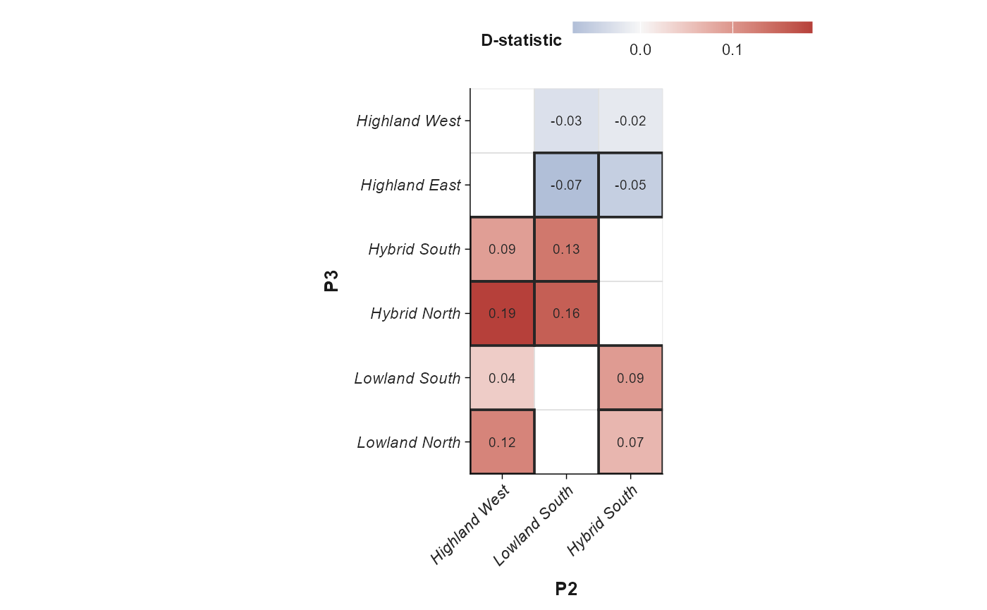

Use style = "trio" when the same Dsuite table should be shown as an ordered forest/lollipop summary. This keeps the sign visible and uses filled points for significant rows.

plot_introgression(dsuite_bbaa, style = "trio")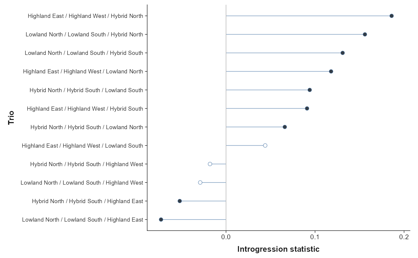

ADMIXTOOLS Statistics

ADMIXTOOLS outputs are statistic tables. qpdstat is imported as stat = "D", f3 as stat = "f3", and f4ratio as stat = "f4_ratio". These should be drawn as trio summaries with standard-error bars when se is present. The example tables use the same highland/lowland/hybrid population set so the forest-style summaries show both significant admixture and near-zero contrasts. Z/P columns are retained in the data rather than being coerced into graph edges. When multiple statistic families are plotted together, ggPopi facets by stat so D-statistics, f3 values, and f4-ratio estimates are not mixed on a single scale.

qpdstat <- import_introgression(
  ggpop_extdata("introgression", "admixtools", "qpdstat_result.csv"),
  type = "admixtools"
)
f3 <- import_introgression(
  ggpop_extdata("introgression", "admixtools", "f3_result.csv"),
  type = "admixtools"
)
f4ratio <- import_introgression(
  ggpop_extdata("introgression", "admixtools", "f4ratio_result.csv"),
  type = "admixtools"
)
unique(qpdstat$stat)
#> [1] "D"
unique(f3$stat)
#> [1] "f3"
unique(f4ratio$stat)
#> [1] "f4_ratio"

plot_introgression(qpdstat)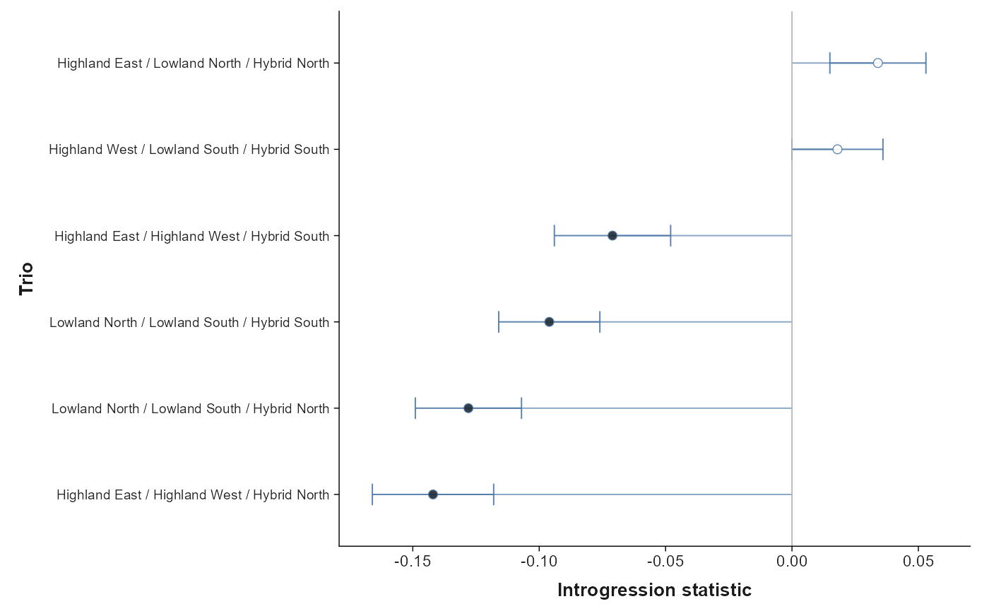

admixtools_all <- import_introgression(
  ggpop_extdata("introgression", "admixtools"),
  type = "admixtools"
)
plot_introgression(admixtools_all)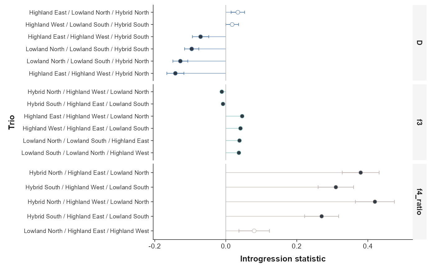

TreeMix Edge Summaries

TreeMix full plotting requires its own tree layout and covariance residual logic. In this module, TreeMix internal *.edges.gz and *.treeout.gz outputs are imported as a compact graph summary so migration and tree edges can still be inspected in the same tidy workflow. When a matching *.vertices.gz file is available next to an *.edges.gz file, import_introgression() uses it to keep the TreeMix drift-coordinate layout instead of falling back to a generic graph. The lightweight graph labels population tips only; internal TreeMix node identifiers are kept out of the display.

treemix_edges <- import_introgression(
  ggpop_extdata("introgression", "treemix", "treemix.M1.edges.gz"),
  type = "treemix"
)
table(treemix_edges$stat)
#> 
#> migration      tree 
#>         1         7

plot_introgression(treemix_edges)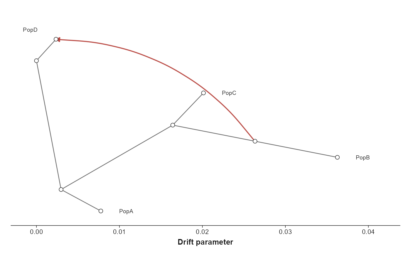

Covariance residual heatmaps, migration-model comparison, and full TreeMix diagnostics are intentionally left for a dedicated TreeMix API rather than being folded into the generic introgression layer.

Layered Path

Use ggpop() plus geom_introgression() when composing with additional ggplot layers.

dsuite_windows |>
  ggpop() +
  geom_introgression(stat = "D")