Ne history • ggPopi

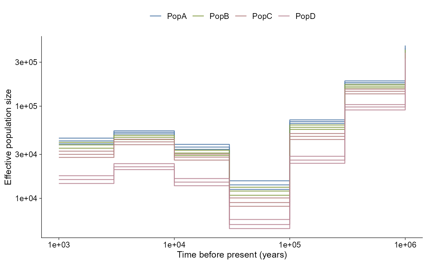
ggpop imports effective population size histories into a typed ggpop_ne_history object. The module supports PSMC, MSMC2, SMC++, and Stairway Plot 2 outputs.

Raw VCF and pop_group.txt metadata are upstream inputs for these external demographic inference tools. ggPopi reads their output tables; it does not estimate Ne histories directly from VCF.

API summary

Task	API	Notes
Import PSMC	`import_ne_history(file, type = "psmc")`	Scaled by default; pass `mutation_rate` for absolute values
Import MSMC2	`import_ne_history(file, type = "msmc2")`	Reads final output with time boundaries and lambda columns
Import SMC++	`import_ne_history(file, type = "smcpp")`	Reads `smc++ plot --csv` output (`label,x,y,plot_type,plot_num`)
Import Stairway Plot 2	`import_ne_history(file, type = "stairway")`	Reads `.summary` output with `year`, `Ne_median`, and percentile columns
Direct plot	`plot_ne_history(data)`	Returns a `ggplot` object
Layered plot	`ggpop(data) + geom_ne_history()`	Tidy ggplot extension path

import_demographic_history(), plot_demographic_history(), and geom_demographic_history() are aliases for the same API. They are provided for users who think in demographic-history terms rather than Ne-history terms.

Plot conventions

plot_ne_history() defaults to the plotting style used most often by each upstream workflow. SMC++ fitted histories are drawn as curves. PSMC, MSMC2, and Stairway Plot 2 histories are drawn as step curves because their native outputs represent piecewise time intervals. Time and Ne axes are log-scaled by default, matching the usual demographic-history presentation; pass log_x = FALSE or log_y = FALSE for linear axes.

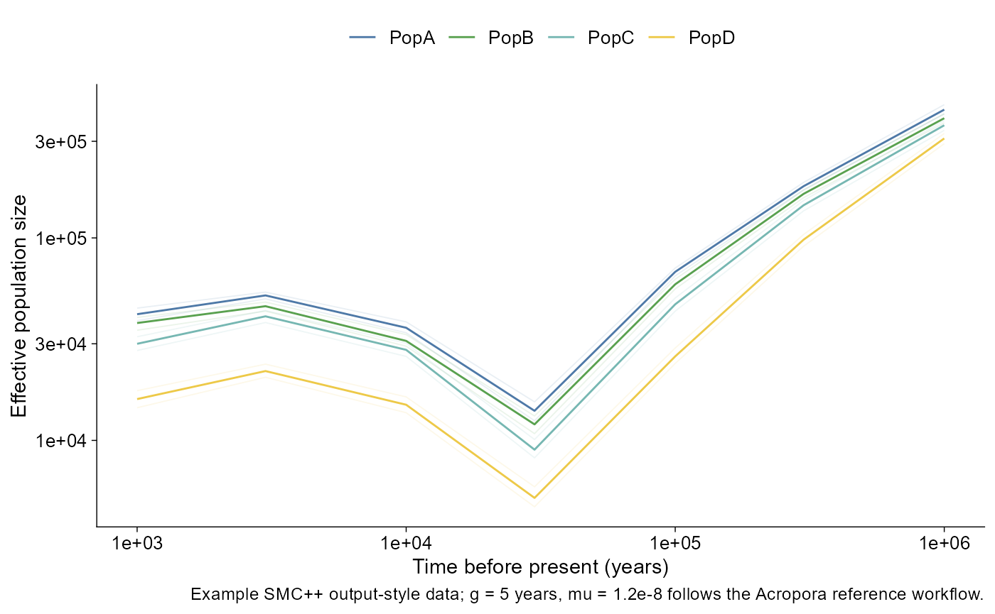
SMC++ curves

The bundled SMC++ example follows the Acropora-style CSV shape label,x,y,plot_type,plot_num, extended with population labels from pop_group.txt (PopA-PopD) and bootstrap trajectories. Values are biologically plausible output-like examples: a recent recovery, a bottleneck around tens of thousands of years ago, and larger ancestral Ne. They are not estimated inside ggPopi.

smcpp <- import_ne_history(
  ggpop_extdata("ne_history", "SMC++", "model.csv"),
  type = "smcpp",
  mutation_rate = 1.2e-8,
  generation_time = 5
)
class(smcpp)
#> [1] "ggpop_ne_history" "data.frame"
head(smcpp)
#>   method sample_id  time     ne time_unit    scale      file
#> 1  SMC++      PopA 1e+03  42000     years absolute model.csv
#> 2  SMC++      PopA 3e+03  52000     years absolute model.csv
#> 3  SMC++      PopA 1e+04  36000     years absolute model.csv
#> 4  SMC++      PopA 3e+04  14000     years absolute model.csv
#> 5  SMC++      PopA 1e+05  68000     years absolute model.csv
#> 6  SMC++      PopA 3e+05 180000     years absolute model.csv
#>   mutation_rate generation_time type plot_type plot_num replicate
#> 1       1.2e-08               5 main      path        0          
#> 2       1.2e-08               5 main      path        0          
#> 3       1.2e-08               5 main      path        0          
#> 4       1.2e-08               5 main      path        0          
#> 5       1.2e-08               5 main      path        0          
#> 6       1.2e-08               5 main      path        0          
#>   source                  .group
#> 1  smcpp SMC++:PopA:main:path:0:
#> 2  smcpp SMC++:PopA:main:path:0:
#> 3  smcpp SMC++:PopA:main:path:0:
#> 4  smcpp SMC++:PopA:main:path:0:
#> 5  smcpp SMC++:PopA:main:path:0:
#> 6  smcpp SMC++:PopA:main:path:0:

plot_ne_history(
  smcpp,
  caption = "Example SMC++ output-style data; g = 5 years, mu = 1.2e-8 follows the Acropora reference workflow."
)

Effective population size history line plot. Time before present is on the x-axis and effective population size is on the y-axis, with separate curves for four populations. Bootstrap trajectories are faint lines behind the main population curves.

SMC++ CSV files produced on a generation scale can be converted to years by passing generation_time. If the input already has a time_unit column set to years, the x values are left unchanged.

Stairway Plot 2 intervals

Stairway Plot 2 summaries often contain lower and upper interval estimates. When ne_lower and ne_upper are available, plot_ne_history() draws a light confidence ribbon around the step curve, matching the usual Stairway Plot summary display of an estimate with interval bounds.

stairway <- import_ne_history(
  ggpop_extdata("ne_history", "StairwayPlot2", "summary.txt"),
  type = "stairway",
  sample_id = "Stairway"
)
plot_ne_history(stairway, ci = TRUE)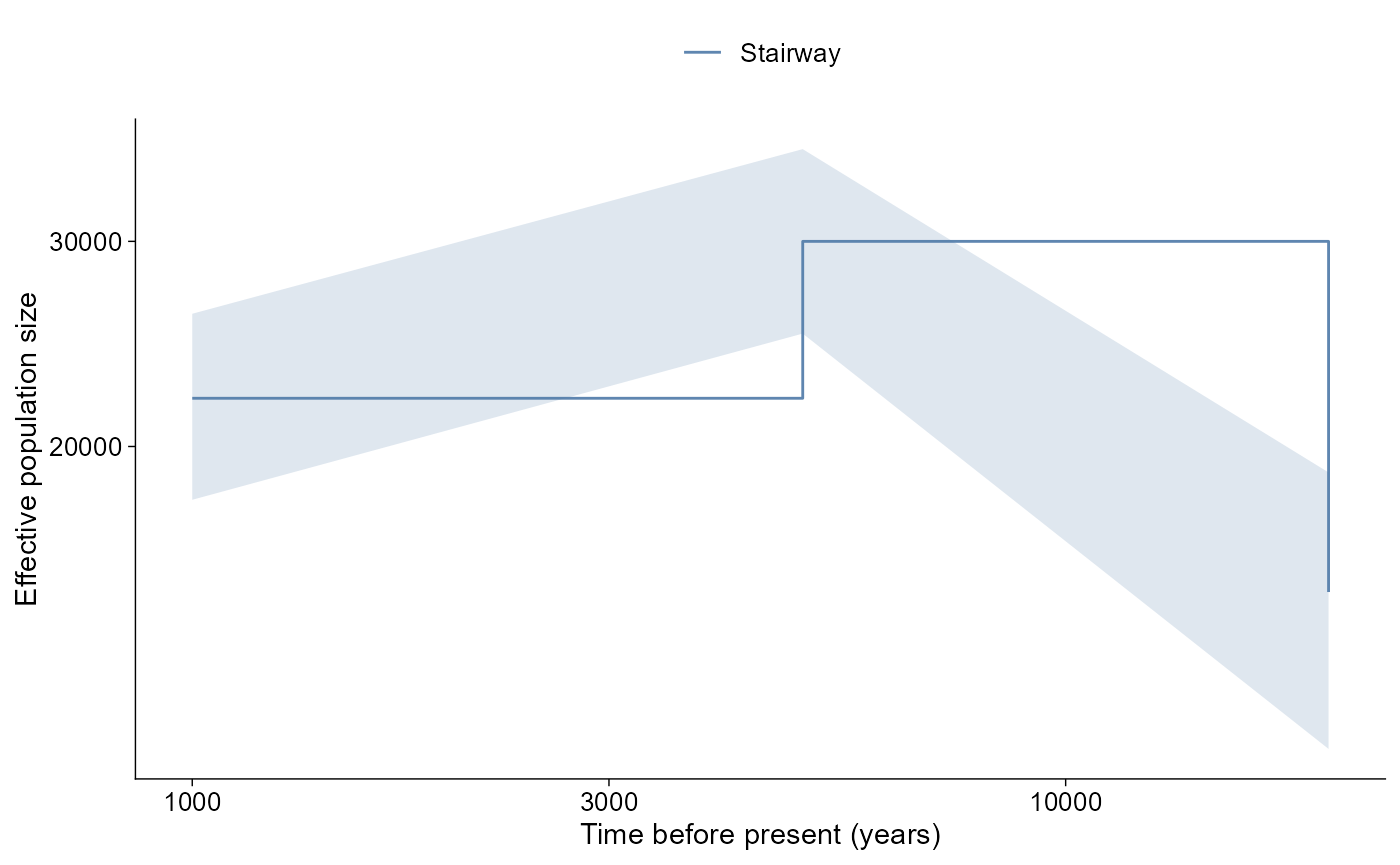

Effective population size history with a confidence ribbon. The median Ne curve is shown through time and a translucent band marks lower and upper estimates.

PSMC and MSMC2 scaling

PSMC and MSMC2 outputs are scaled unless a mutation rate is supplied. Passing mutation_rate converts to absolute Ne and time; generation_time can then convert generations to years. Their default plot style is a step curve, which matches the interval-based output used by psmc_plot.pl and MSMC plotting helpers.

psmc_scaled <- import_ne_history(
  ggpop_extdata("ne_history", "PSMC", "sample.psmc"),
  type = "psmc",
  sample_id = "PSMC"
)
unique(psmc_scaled$scale)
#> [1] "relative"

msmc_absolute <- import_ne_history(
  ggpop_extdata("ne_history", "MSMC2", "final.txt"),
  type = "msmc2",
  sample_id = "MSMC2",
  mutation_rate = 1e-8
)
unique(msmc_absolute$scale)
#> [1] "absolute"

plot_ne_history(msmc_absolute)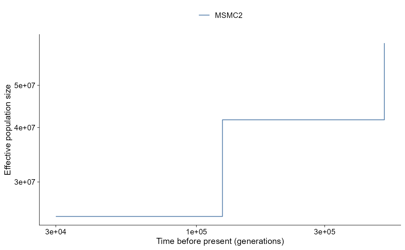

MSMC2 effective population size history as a step curve. Time before present is log-scaled on the x-axis and effective population size is on the y-axis.

Layered path

Use ggpop() plus geom_ne_history() when composing with additional ggplot layers.

smcpp |>
  ggpop() +
  geom_ne_history()

Layered Ne history plot using ggpop plus geom_ne_history. Population-specific SMC++ curves are drawn on log-scaled time and Ne axes.